Who's onlineThere are currently 0 users and 3 guests online.
User loginBook navigationNavigationLive Traffic MapNew Publications
|
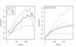
Fig. 5.15: Anisotropy (left) and variogram model fitted using the Maximum Likelihood (ML) method (right). and variogram model fitted using the Maximum Likelihood (ML) method (right).")
data(meuse)
coordinates <- ~x+y
zinc.geo <- as.geodata(meuse["zinc"])
str(zinc.geo)
# plot(zinc.geo)
# Variogram modelling (target variable):
par(mfrow=c(1,2))
# anisotropy ("lambda=0" indicates log-transformation):
plot(variog4(zinc.geo, lambda=0, max.dist=1500, messages=FALSE), lwd=2)
# fit variogram using likfit:
zinc.svar2 <- variog(zinc.geo, lambda=0, max.dist=1500, messages=FALSE)
zinc.vgm2 <- likfit(zinc.geo, lambda=0, messages=FALSE, ini=c(var(log1p(zinc.geo$data)),500), cov.model="exponential")
zinc.vgm2
# this carries much more information!
env.model <- variog.model.env(zinc.geo, obj.var=zinc.svar2, model=zinc.vgm2)
plot(zinc.svar2, envelope=env.model); lines(zinc.vgm2, lwd=2);
legend("topleft", legend=c("Fitted variogram (ML)"), lty=c(1), lwd=c(2), cex=0.7)
dev.off()
|
Latest image Testimonials"Hi Tom. I have uploaded some comments on your book. You should check if you are able to run the code on upgraded versions of R. Otherwise fine, nice set of full-scale examples." PollRandom image |
 | Contact: Tomislav Hengl ([email protected]) |
Recent comments
8 years 5 weeks ago
8 years 22 weeks ago
8 years 30 weeks ago
8 years 43 weeks ago