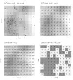
 species distribution maps produced using common statistical models.")
library(geoR)
library(spatstat)
set.seed(312)
cp <- expand.grid(seq(0, 1, l=10), seq(0, 1, l=10))
# unconditional gaussian simulations (psill=1, mean=0):
s <- grf(100, grid="reg", cov.pars=c(1, 0.2), cov.model="mat", kappa=1.5)
hist(s$data)
# define your own model, e.g. poisson:
lambda <- 0.2*exp(0.5 +s$data)
y <- rpois(length(s$data), lambda=lambda)
image(s, col=gray(seq(1, 0.5, l=21)))
text(s$coords, label=y, pos=3, offset=-0.2, cex=1.5)
hist(y)
dev.off()
# simulate a point pattern:
sm <- list(x=seq(0, 1, l=10), y=seq(0, 1, l=10), z=matrix(y, nrow=10))
y.p <- rpoint(n=sum(y), f=as.im(sm))
image(s, col=gray(seq(1, 0.5, l=21)))
points(y.p, pch="+", cex=1.5)
# yes/no events:
y.b <- ifelse(y>0, 1, 0)
sb <- s
sb$data <- y
image(sb, col=gray(c(0.95,rep(0.5, 10))))
text(s$coords, label=y.b, pos=3, offset=-0.2, cex=1.5)
# binomial model:
p <- exp(0.1+s$data)/(1+exp(0.1+s$data))
y <- rbinom(length(s$data), size=100, prob=p)/100
image(s, col=gray(seq(1, 0.5, l=21)))
text(s$coords, label=y, pos=3, offset=-0.2, cex=1.2)
hist(y)
dev.off()
# bernoulli model:
p <- 0.2*exp(s$data)/(1+exp(s$data))
ind <- seq(1, 401, by=8)
y <- rbinom(length(s$data), size=1, prob=p)
y <- rbinom(p[ind], size=1, prob=p)
image(s, col=grey(0.8))
text(s$coords, label=y, pos=3, offset=-0.2, cex=1.5)
hist(y)
# uniform distribution:
y.cdf <- ecdf(s$data)
y <- y.cdf(s$data)
image(s, col=gray(seq(1, 0.5, l=21)))
text(s$coords, label=y, pos=3, offset=-0.2, cex=1.2)
dev.off()
hist(y)

 species distribution maps produced using common statistical models.")
 | Contact: Tomislav Hengl ([email protected]) |
Recent comments
7 years 28 weeks ago
7 years 45 weeks ago
8 years 1 week ago
8 years 14 weeks ago