Least squares fit

Table window	Columns menu
Least Squares Fit

This topic consists of the following sections:

1. Functionality

2. Dialog box

3. Command line

4. Algorithm

5. Description of functions

Functionality

The least squares fit operation calculates for all discrete values in two input columns an output value in an output column, according to a certain user-selected function which is supposed to describe the relation between all values in the two input columns. Coefficients for this function are calculated in such a way that the sum of errors is as small as possible (best fit).

The least squares fit operation provides a tool to describe the best fitting relation between two columns in a table. The most common application of this concept is a linear regression which means the two table columns are known or expected to have some linear relationship.

This may be described with the following equation:

Y = a * X + b

where X and Y are known variables (records from the two columns in the table) and where a and b are unknown coefficients.

Usually there is some experimental error present or other deviation from a line describing the relation between X and Y. This means that no values for a and b are possible for a perfect fit. The best fit is found when the sum of the errors is as small as possible. This is the case when the sum of squares of the deviations of all points from the line, indicating the relationship, is as small as possible (see figures below). In other words the sum of squares of the errors on each data point is minimized.

The model used, provides a method for finding the least squares approximation to a set of data points (X, Y). The approximation must be a linear combination of a set basis vectors. The functional form of the approximation (polynomial, exponential etc.) is determined by the user.

To find the least squares fit, X and Y can be represented graphically using one of the five predefined function types: exponential, logarithmic, power law, polynomial or trigonometric.

Then the number of terms can be specified:

when using 2 terms in a polynomial function, the function will read:

Y = aX + b

when using 3 terms in a polynomial function, the function will read:

Y = aX² + bX + c

etc.

By calculating a least squares fit through the Columns menu of a table window, you will thus obtain values in an output column which if plotted in a graph are positioned exactly on the line which represents the best fitting curve through all input points.

Tip:

It might be easier to directly calculate a least squares fit in a graph window.

First, create a graph from two columns in a table.
Then, in the graph window, choose Add Graph Least Squares Fit from the Edit menu of the graph window;
In the appearing Add Graph Least Squares Fit dialog box, select the two input columns again, and select a function how the least squares fit should be calculated.

The results of the least squares fit will then be directly shown as a continuous line in your graph window. The resulting formula can be viewed in the Graph Options - Least Squares Fit dialog box; in this dialog box you can also modify the calculation by choosing another function, etc.

Examples:

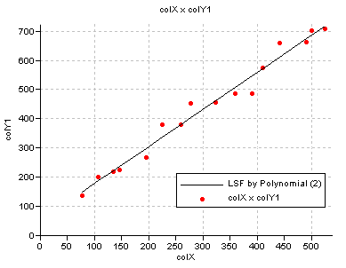
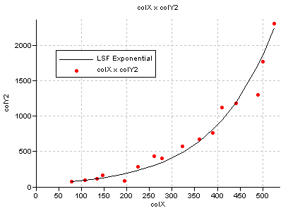
The examples below show the relations between column colX and column colY1 and between column colX and column colY2 as a result of a least squares fit.

Fig. 1: The best fit between colX and colY1 using a polynomial function with 2 terms (a straight line) defined by the line:
Y = 49.101 + 1.276 * X

Fig. 2: The best fit between colX and colY2 using an exponential function (always 2 terms) defined by the line:
Y = 42.341302790409 * exp(0.007566547732 * X)

When using the least squares fit operation on the Columns menu of a table window, the output column shows the Y-values which are exactly on the line of the best-fit curve.

Input column requirements:

The input columns should both have a value domain.
The number of points should be at least 2; points having undefined values for X and/or Y included.
The exponential function require that all Y-values have the same sign (either all positive, or all negative) and none of them equals 0.
The logarithmic function requires that all X-values have the same sign (either all positive, or all negative) and none of them equals 0.
The power law function requires that all X-values are positive and that the Y-values all have the same sign (either all positive or all negative) and none of them equals 0.
The trigonometric ('Fourier') function requires at least 3 terms.
The number of points must be at least equal to the number of terms selected (undefineds not counted).

Dialog box

The least squares fit operation provides a tool to describe the best fitting relation between two table columns. Usually there is some experimental error present or other deviation from a line describing the relation between X and Y. This means that no values for a and b are possible for a perfect fit. The best fit is found when the sum of the errors (least squares) is as small as possible.

Dialog box options:

X - column:	Select the name of the column representing the x-values (independent variable). For the input column requirements, see above Functionality.
Y - column:	Select the name of the column representing the y-values (dependent variable).
Function:	Select the type of function: Exponential, Logarithmic, Polynomial, Power Law, or Trigonometric. For more information, see Functionality and Algorithm.
Nr. of terms:	Type the number of terms to be used in the formula, describing the best fit. The text box is only available for function types polynomial (minimum 2 terms) and trigonometric (minimum 3 terms).
Output column:	Type the name of the output column that will contain the transformed Y-values (obtained by applying the fitting function to the independent (X) variable, skipping undefined values). A dependent column is created.

The Column Properties dialog box appears.

Tips:

To view the resulting least squares fit formula: double-click the output column name in the table. The Column Properties dialog box appears; then, click the Additional Info button in that dialog box.

To view the results in a graph, choose the Create Graph command from the File menu in the table window.

To display the input values as points:

for the X-axis of the graph, use the same column as you used as input X in the least squares fit;
for the Y-axis of the graph, use the same column as you used as input Y in the least squares fit;

A point graph will be directly shown.

To display the results of the least-squares fit as a line:

From the Edit menu in the graph window, choose Add Graph from Columns;
In the appearing Add Graph from Columns dialog box:

for the X-axis of the graph, select the same X-column as you used in the least squares fit;
for the Y-axis of the graph, select the output column of the least squares fit;

Initially, a point graph will be displayed.

Then, double-click this graph layer in the Graph Management pane. In the appearing Graph Options - Graph from Columns dialog box, choose graph type Line.

Now, a line will be drawn through the calculated values.

It is probably easier to directly perform a least squares fit in a graph window.

Create a graph from the input columns, as described above.
In the graph window, choose Add Graph Least Squares Fit from the Edit menu of the graph window;
In the appearing Add Graph Least Squares Fit dialog box, select the two input columns again, and a function how the least squares fit should be calculated.

The results of the least squares fit will then be directly shown as a line in your graph window.

Command line

The Least Squares Fit operation can be directly executed by typing one of the following expressions on the command line of the table window:

OUTCOL	=	ColumnLeastSquaresFit(Col1, Col2, Function)
OUTCOL	=	ColumnLeastSquaresFit(Col1, Col2, Function, n)

where:

OUTCOL	is the name of your output column.
ColumnLeastSquaresFit
	is the command to start the Least Squares Fit operation.
Col1	is the name of your X-column, i.e. an independent variable with a value domain.
Col2	is the name of your Y-column, i.e. a dependent variable with a value domain.
Function	is the function to be used in the description of the relationship between X and Y. For the function, type either: exponential \| logarithmic \| polynomial \| power \| trigonometric
n	When using a polynomial or trigonometric function: Optional parameter to specify the number of terms to be used in the function. n may not be greater than the number of valid data points, excluding points with undefined X or Y values. If the parameter is omitted, 2 terms will be used for a polynomial function, and 3 terms will be used for a trigonometric function. When using an exponential, logarithmic or power function: Parameter is not required and can be omitted: always 2 terms will be used.

When the definition symbol = is used, a dependent output column is created; when the assignment symbol := is used, the dependency link is immediately broken after the column is calculated.

Algorithm

Given a set of m data points (X,Y) and n unknown coefficients in the fitting function, an m * n matrix (m ≥ n), is constructed. In this matrix, n is the number of basis vectors in the approximation. A basis vector is a function itself defined by the fit type, selected by the user. The accuracy of the fit (goodness of fit) is indicated by the standard deviation:

S.D. = Ö ( S (Y_i - F (X_i) )² / (m - n))

where:

F(X_i)	is the least squares solution at the point X_i.
(Y_i - F (X_i))	is the residual and (m - n) is the degree of freedom to the fit.

Description of functions

Exponential:

This module fits the function: Y = a e^b X

where a and b are real numbers to the data points.

A linear equation is obtained by taking the natural logarithm of both sides:

ln(Y) = ln(a) + b X

Note:

The Y-values of the data points must all have the same sign (either all positive or all negative).

Logarithmic:

This module fits the function: Y = a ln(bX)

in which a and b are real numbers to the data points.

A linear equation is obtained rewriting the equation to:

Y = a ln(b) + a ln(X)

Note:

The X-values of the data points must all have the same sign (either all positive or all negative) and none of them equals 0.

Polynomial:

This module uses Chebyshev polynomials to fit a polynomial to the data points.

The Nr of terms must be one greater than the degree of the polynomial. A straight-line least squares fit needs only two terms. The elements of the solution vector S will be as follows:

S_j = a_j

where:

a_j	is the coefficient of X_{j - 1}
1 <= j <= Nr of terms
2 <= Nr of terms <= Nr data points

Power law:

This module fits the function: Y = a X^b

in which a and b are real numbers to the data points.

A linear equation is obtained by taking the natural logarithm of both sides:

ln(Y) = ln(a) + b * ln(X)

Note:

All X-values of the data points must be positive and the Y-values of the data points must all have the same sign (either all positive or all negative) and none of them equals 0.

Trigonometric:

This module fits a finite Fourier series to the data points.

The elements of the solution vector S will be as follows:

S_j = F_{j - 1}

where:

F_{j - 1}	is the (j - 1)^th term in the Fourier series.
1 <= j <= Nr of terms
3 <= Nr of terms <= Nr data points

The first few terms in the Fourier series are:

F₀ = 1

F₁ = cos(X)

F₂ = sin(X)

F₃ = cos(2X)

F₄ = sin(2X)

F₅ = cos(3X)

F₆ = sin(3X)

Table window

Least Squares Fit

Functionality

Dialog box

Command line

Algorithm

Description of functions