Retrieval and analysis of GBIF records in R
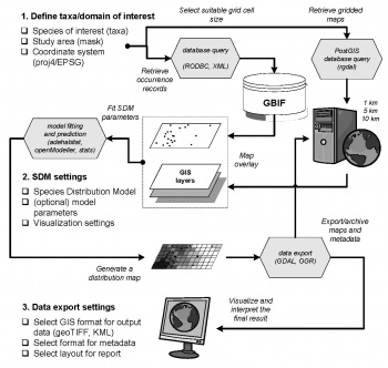
BIF is a growing gateway to global biodiversity data (containing over 180 millions of occurrence records of over 3 millions of differently named taxa; based on the server statistics on August 2009). In this article we demonstrate the ways to automate analysis of the GBIF data (KML one-arcdegree cell density files; original point records) using R environment for statistical computing in combination with open source GIS packages. We focus our analysis on the occurrence records for the list of 495 European breeding birds, in order to determine: (1) which are the dominant bird species? (2) which species are spatially correlated? (3) where are the biodiversity hot-spots? and (4) can the detail of the existing maps be improved using finer-resolution environmental maps? For more details about this topic consider obtaining the original article:
- Hengl, T., Saarenmaa, H. 2010? Automated retrieval and analysis of GBIF records in R: some examples with European breeding birds.
Global Ecology and Biogeography, in progress.
|
Contents |
Download of the GBIF one-degree density maps
We initially need to define the bulk of species of interest for biogeographic analysis. We simply copy the species listed at the EBCC Atlas website using the url method of the base package.
> ebcc.url <- htmlTreeParse("http://www.sovon.nl/ebcc/")
> bird.n <- length(ebcc.url$children$html[[2]][[2]][[2]][[1]][[13]])-1
> bird.list <- as.list(rep(NA, bird.n))
# copy the names from EBCC:
> for(i in 1:bird.n){
>  bird.list[[i]] <- as.character(ebcc.url$children$html
+     [[2]][[2]][[2]][[1]][[13]][[i+1]][[1]])[6]
> }
> bird.list[1:5]
[[1]]
[1] "Accipiter brevipes"

[[2]]
[1] "Accipiter gentilis"

[[3]]
[1] "Accipiter nisus"

[[4]]
[1] "Acridotheres cristatellus"

[[5]]
[1] "Acridotheres tristis"
In the following step, we need to match the species name with the GBIF ID --- the unique 8-digit number assigned by GBIF. The GBIF Data Portal offers an XML-based API service to retrieve the default taxonomy, root taxa, ID number etc. For example, to determine the ID of species Accipiter brevipes, we can use:
# Match the Scientific names and IDs:
> gbif.id <- as.list(rep(NA, bird.n))
> for(i in 1:bird.n){
>  gbif.url <- url(paste("http://data.gbif.org/species/nameSearch?query=",
+    strsplit(bird.list[[i]]," ")[[1]][1],"%20",
+    strsplit(bird.list[[i]]," ")[[1]][2],"&maxResults=1&returnType=nameId",sep=""), blocking=F)
>  gbif.id[[i]] <- ifelse(is.null(scan(gbif.url, what="integer", quiet=T, n=1)),
+    NA, scan(gbif.url, what="character", quiet=T, n=1)[1])
>  close(gbif.url)
> }  # this can take (A LOT OF) time!
> gbif.id[1:5]
[[1]]
[1] "13849996"

[[2]]
[1] "13832791"

[[3]]
[1] "13832394"

[[4]]
[1] "13815858"

[[5]]
[1] "13837229"
Once we have determined the GBIF ID numbers for our list of species, we can proceed with obtaining the KML one-arcdegree cell densities. Each species has a standard URL e.g.:
# Download the occurrence data (celldensity) from the Google Earth overlay:
> for(i in 1:bird.n){
> system(paste('"c:/Program Files/firefox/firefox.exe" -remote
+     openURL("http://data.gbif.org/occurrences/taxon/celldensity/taxon-celldensity-',
+     gbif.id[[i]],'.kml")',sep=""))
 # simple download.file did not run --- server blocking?
 # download.file(paste("http://data.gbif.org/occurrences/taxon/celldensity/taxon-celldensity-",
 # +    gbif.id[[i]],".kml",sep=""), destfile=paste(getwd(),"/taxon-celldensity-",
 # +    gbif.id[[i]],".kml",sep=""))
> }
To actually read all downloaded KML files in R, we need to read them as XML files, locate the position of coordinates (grid nodes), then copy the values of coordinates and density counts to a table:
# list all downloaded files and convert them to ILWIS format:
> gbif.grid <- list.files(getwd(), pattern="\\.kml$", recursive=T, full=F)
> gbif.sp <- as.list(rep(NA, length(gbif.grid)))
> levels(gbif.grid) <- list.files(getwd(), pattern="\\.kml$", recursive=T, full=F)

# convert to a SpatialPointsDataFrame:
> for(i in 1:length(gbif.grid)){
>  id <- strsplit(strsplit(gbif.grid[[i]], "-")[[1]][3], ".kml")[[1]]
>  tmp <- xmlTreeParse(gbif.grid[[i]])
>  lengthp <- length(tmp$doc[[1]])-4
>  GBIF_sp <- data.frame(Longitude=rep(0,lengthp), Latitude=rep(0,lengthp),
+       Count=rep(0,lengthp))
>  for(j in 1:lengthp) {
>    if(!is.null(tmp$doc[[1]][j+4][[1]][2][[1]][5][[1]][[1]][[1]])){
>     LatLon <- unclass(tmp$doc[[1]][j+4][[1]][2][[1]][5][[1]][[1]][[1]])$value
>     Countx <- unclass(tmp$doc[[1]][j+4][[1]][2][[1]][1][[1]][[1]])$value
>     GBIF_sp$Longitude[[j]] <- as.numeric(matrix(unlist(strsplit(LatLon, split=",")), ncol=3)[1])
>     GBIF_sp$Latitude[[j]] <- as.numeric(matrix(unlist(strsplit(LatLon, split=",")), ncol=3)[2])
>     GBIF_sp$Count[[j]] <- as.numeric(matrix(unlist(strsplit(Countx, split=" ")), ncol=5)[4])
>   }}
>  if(length(GBIF_sp$Count)>0){
>  coordinates(GBIF_sp) <-~Longitude+Latitude
>  proj4string(GBIF_sp) <- CRS("+proj=longlat +ellps=WGS84")
# copy temp object:
>  gbif.sp[i] <- GBIF_sp
>  }
>  rm(GBIF_sp)
> }
> save(gbif.sp, file="gbif_pnt.Rdata")
> str(gbif.sp[[1]])
Formal class 'SpatialPointsDataFrame' [package "sp"] with 5 slots
  ..@ data       :'data.frame': 31 obs. of  1 variable:
  .. ..$ Count: num [1:31] 3 3 1 3 1 1 1 3 5 1 ...
  ..@ coords.nrs : int [1:2] 1 2
  ..@ coords     : num [1:31, 1:2] 35.5 102.5 90.5 100.5 106.5 ...
  .. ..- attr(*, "dimnames")=List of 2
  .. .. ..$ : NULL
  .. .. ..$ : chr [1:2] "Longitude" "Latitude"
  ..@ bbox       : num [1:2, 1:2] 11.5 33.5 108.5 65.5
  .. ..- attr(*, "dimnames")=List of 2
  .. .. ..$ : chr [1:2] "Longitude" "Latitude"
  .. .. ..$ : chr [1:2] "min" "max"
  ..@ proj4string:Formal class 'CRS' [package "sp"] with 1 slots
  .. .. ..@ projargs: chr " +proj=longlat +ellps=WGS84"
so that the object now shows spatial (sp) structure with five slots: (1) the attribute table, (2) spatial dimensions, (3) coordinates of points, (4) bounding box of the map, and (5) proj4 coordinate system definition (for more info how are spatial objects defined in R see Bivand et al. (2008). This shows that the species Accipiter brevipes, according to the GBIF Data Portal, occurs at only 31 grid nodes.
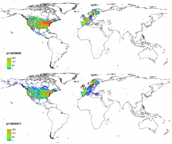
Now that we have organized the distribution maps, we can do some sorting, for example, to determine the species with highest geographical spreading:
> spred.list <- data.frame(gbif.id=levels(gbif.grid), total=rep(0,length(levels(gbif.grid))))
> for(i in 1:length(sum.list$gbif.id)){
>    if(!is.na(gbif.sp[i])){
>    spred.list[i,2] <- length(gbif.sp[[i]]@data[[1]])
> }}
> spred.list[1:5,]
                         gbif.id total
1 taxon-celldensity-13791657.kml    31
2 taxon-celldensity-13791658.kml    52
3 taxon-celldensity-13791659.kml   120
4 taxon-celldensity-13791661.kml   345
5 taxon-celldensity-13791696.kml  1120
We can convert the point map to a gridded map using the functionality of the open source GIS SAGA (RSAGA package communicates operations from R to SAGA):
> gbif.gridded <- as.list(rep(NA, length(gbif.grid)))
> for(i in 1:length(gbif.sp)){
>  if(!is.na(gbif.sp[i])){
>   id <- strsplit(strsplit(gbif.grid[[i]], "-")[[1]][3], ".kml")[[1]]
>  unlink("GBIF_sp.???")
>  writeOGR(gbif.sp[[i]]["Count"], "GBIF_sp.shp", "GBIF_sp", "ESRI Shapefile")
>  rsaga.geoprocessor(lib="grid_gridding", module=3, param=list(GRID="GBIF_sp.sgrd",
+      INPUT="GBIF_sp.shp", FIELD=0, LINE_TYPE=0, USER_CELL_SIZE=1,
+      USER_X_EXTENT_MIN=-179.5, USER_X_EXTENT_MAX=179.5, USER_Y_EXTENT_MIN=-89.5,
+      USER_Y_EXTENT_MAX=89.5))
>  rsaga.sgrd.to.esri(in.sgrds="GBIF_sp.sgrd", out.grids=
+      set.file.extension(paste("pr",id,sep=""),".asc"), out.path=getwd(), prec=0)
>  unlink("GBIF_sp.???")
> }}
where rsaga.geoprocessor is a generic command to send an operation from R to SAGA, arguments GRID and INPUT define the input shape file and output grid file, FIELD defines spatial attribute of interest (density values in this case), USER_CELL_SIZE and USER_CELL_EXTENT are used to define the grid system. To get a full description of each SAGA module, you can use (Brenning, 2008):
> rsaga.get.usage(lib="grid_gridding", module=3)
SAGA CMD 2.0.3
library path:   C:/Progra~1/saga_vc/modules
library name:   grid_gridding
module name :   Natural Neighbour
Usage: 3 [-GRID <str>] -SHAPES <str> [-FIELD <num>] [-TARGET <num>] [-SIBSON]
[-USER_CELL_SIZE <str>] [-USER_FIT_EXTENT] [-USER_X_EXTENT_MIN <str>]
[-USER_X_EXTENT_MAX <str>] [-USER_Y_EXTENT_MIN <str>] [-USER_Y_EXTENT_MAX <str>]
[-SYSTEM_SYSTEM_NX <num>] [-SYSTEM_SYSTEM_NY <num>] [-SYSTEM_SYSTEM_X <str>]
 [-SYSTEM_SYSTEM_Y <str>] [-SYSTEM_SYSTEM_D <str>] [-GRID_GRID <str>]
  -GRID:<str>                   Grid
        Data Object (optional output)
  -SHAPES:<str>                 Points
        Shapes (input)
  -FIELD:<num>                  Attribute
        Table field
  -TARGET:<num>                 Target Grid
        Choice
        Available Choices:
        [0] user defined
        [1] grid system
        [2] grid
  -SIBSON                       Sibson
        Boolean
  -USER_CELL_SIZE:<str>         Grid Size
        Floating point
        Minimum: 0.000000
  -USER_FIT_EXTENT              Fit Extent
        Boolean
  -USER_X_EXTENT_MIN:<str>      X-Extent
        Value range
  -USER_X_EXTENT_MAX:<str>      X-Extent
        Value range
  -USER_Y_EXTENT_MIN:<str>      Y-Extent
        Value range
  -USER_Y_EXTENT_MAX:<str>      Y-Extent
        Value range
  -SYSTEM_SYSTEM_NX:<num>       Grid System
        Grid system
  -SYSTEM_SYSTEM_NY:<num>       Grid System
        Grid system
  -SYSTEM_SYSTEM_X:<str>        Grid System
        Grid system
  -SYSTEM_SYSTEM_Y:<str>        Grid System
        Grid system
  -SYSTEM_SYSTEM_D:<str>        Grid System
        Grid system
  -GRID_GRID:<str>              Grid
Import of KML files and their conversion to ArcInfo ASCII grids can be automated by looping the commands from above using a list of species. Once we have generated ArcInfo ASCII files for all species, we can read them back to R using the rgdal package:
# Import back all maps to R:
> asc.list <- list.files(getwd(), pattern="\\.asc$", recursive=T, full=F)
> levels(asc.list) <- list.files(getwd(), pattern="\\.kml$", recursive=T, full=F)
> gbif.gridded <- readGDAL(asc.list[1])
> gbif.gridded$band1 <- ifelse(gbif.gridded$band1<0, NA, gbif.gridded$band1)
> names(gbif.gridded)[1] <- sub(".asc", "", asc.list[[1]])
> for(i in asc.list[-1]) {
>    tmp <- readGDAL(paste(i))$band1
>    gbif.gridded@data[sub(".asc", "", i[[1]])] <- ifelse(tmp<0, NA, tmp)
> }
> str(names(gbif.gridded))
chr [1:426] "pr13791657" "pr13791658" "pr13791659" ...
> proj4string(gbif.gridded) <- CRS("+proj=longlat +datum=WGS84")
where gbif.gridded is a SpatialGridDataFrame class object consisting of 425 grids. The number is reduced because not all species are available in GBIF; not all available species have at least one record.
PCA / Extraction of Biodiversity index
We are further interested to see if the species with highest geographical coverage are spatially correlated. Once all the maps are put on the same grid, we can run a variety of statistical analysis --- for example principal component analysis (PCA) (Venables and Ripley, 2002):
# convert to a point map:
> pointmaps <- as(gbif.gridded, "SpatialPointsDataFrame")
# insert sof-zeros where NA's:
> for(i in 1:length(pointmaps@data)){
>  pointmaps@data[[i]] <- ifelse(is.na(
+   pointmaps@data[[i]]), 0,
+   pointmaps@data[[i]])
}
> pc.top6 <- prcomp(~pr13837470+pr13810676+pr13809817+pr13839800+pr13810132+pr13837221,+ scale=F, pointmaps, na.action=na.omit) > biplot(pc.top6, xlabs=rep("+", length(pc.top6$x[,1])), xlim=c(-0.05,0.5), ylim=c(-0.15,0.4))
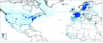
Once we have prepared all density maps for use in a GIS, we can proceed with estimating ecological indices. Our main concern is the derivation of the Biodiversity (Shannon) Index. We start by estimating the total number of species and the total number of occurrences per pixel per species:
# (there are too many species, reduce to 150)
> sum.list <- data.frame(gbif.id=names(gbif.gridded), total=rep(0,length(names(gbif.gridded))))
> for(i in 1:length(sum.list$gbif.id)){
    sum.list[i,2] <- sum(gbif.gridded@data[i], na.rm=T)
> }
> sum.list$rankn <- rank(sum.list$total, ties.method="first")
> top150 <- subset(sum.list, sum.list$rankn>300)
> top150.gridded <- gbif.gridded[as.character(top150$gbif.id)]
# total number of occurrences per grid node:
> top150.gridded$Nsum <- rowSums(top150.gridded@data, na.rm=T, dims=1)
The BI can then be derived by using:
> biodiv <- pointmaps
> for(i in 1:length(pointmaps@data)){
>    biodiv@data[[i]] <- pointmaps@data[[i]]/top150$total[i]*log(pointmaps@data[[i]]/top150$total[i])
> }
> biodiv$BI <- -1*rowSums(biodiv@data, na.rm=T, dims=1)
> summary(biodiv$BI)
     Min.   1st Qu.    Median      Mean   3rd Qu.      Max.
1.446e-05 3.390e-04 2.265e-03 9.255e-02 1.570e-02 1.917e+01
The BI is increased either by having additional unique species, or by having a greater species evenness.
Species' distribution modeling using GBIF records and auxiliary maps
We will now demonstrate some standard species distribution analysis steps using the point records of Sturnus vulgaris. For practical reasons, we will focus on a single country (USA), and on the occurrence records <10 years old. Unfortunately, GBIF absolutely limits download of occurrence records (10,000), so that not the whole of the country can be obtained from the server. To avoid this limitation, we have instead downloaded the original records of Sturnus vulgaris directly from the the Avian Knowledge Network (AKN distributes occurrence records data from bird-monitoring, bird-banding, and broad-scale citizen-based bird-surveillance programs), which is the original data provider of the records to GBIF and sets no limits considering the access to data. We can read these records to R by using:
> AKN <- read.table("AKN_Query_Results_1522009113212.txt")
> str(AKN)
'data.frame':   183289 obs. of  8 variables:
 $ Global.Unique.Identifier: Factor w/ 183288 levels
 $ Longitude           : num  -76.3 -88.2 -124.2 ...
 $ Latitude            : num  36.9 42.3 40.4 ...
 $ Observation.Count   : int  NA NA 34 3 1 1 ...
 $ Observation.Date    : Factor w/ 61531 levels
 $ Year.Collected      : int  2004 2003 2000 ...
 $ Month.Collected     : int  10 7 6 6 6 4 11 ...
 $ Locality            : Factor w/ 34984 levels
This gives us a total of 183,289 of records of Sturnus vulgaris in USA in the last 10 years. The raw records (point observations) first need to be converted to a spatial layer, and reprojected to the local coordinate system:
# mask summer months and observations without LonLat:
> AKN.pnt <- subset(AKN, !is.na(AKN$Longitude)
+    &!is.na(AKN$Latitude)&AKN$Month.Collected>4
+    &AKN$Month.Collected<9)
# attach coordinates / CRS:
> coordinates(AKN.pnt) <- ~Longitude+Latitude
> proj4string(AKN.pnt) <- CRS("+proj=longlat +datum=WGS84")
# reproject to local system:
> AKN.pnts <- spTransform(AKN.pnt, CRS("+proj=aea +lat_1=29.5 +lat_2=45.5 +lat_0=23
+    +lon_0=-96 +x_0=0 +y_0=0 +ellps=GRS80 +datum=NAD83 +units=m +no_defs"))
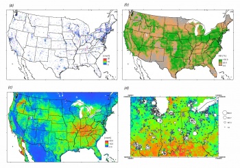
where +proj=aea ... is the Albers equal-area coordinate system commonly used to show the whole of USA. The occurrence records (attribute Observation.Count) are displayed in Fig. below.
We now examine if the spatial distribution of this species can be explained using environmental predictors. For this purpose we use a compendium of 10~km (3600x1300 pixels) publicly available global maps. After we download the maps locally, we can subset the area of interest and reproject the rasters at the same time by using the proj4 module in SAGA GIS:
> rsaga.geoprocessor(lib="pj_proj4", 2, param=list(SOURCE_PROJ="\"+proj=longlat +datum=WGS84\"",
+   TARGET_PROJ="\"+proj=aea +lat_1=29.5 +lat_2=45.5 +lat_0=23 +lon_0=-96 +x_0=0 +y_0=0 +ellps=GRS80
+   +datum=NAD83 +units=m +no_defs\"", SOURCE="biocl01.sgrd", TARGET="m_biocl01.sgrd",
+   TARGET_TYPE=2, INTERPOLATION=1, GET_SYSTEM_SYSTEM_NX=470, GET_SYSTEM_SYSTEM_NY=296,
+   GET_SYSTEM_SYSTEM_X=-2405000, GET_SYSTEM_SYSTEM_Y=265000, GET_SYSTEM_SYSTEM_D=10000))
which will reproject the map of the mean annual temperature to Albers equal-area coordinate system (USA only: 10 km grid; 470[[Image:|LaTeX: %5Ctimes]]296 pixels). In practice, this operation is also run in a loop to a list of maps selected by the user.
Now that we have prepared both point and gridded data, we can proceed with the species distribution modeling. We first focus on the derivation of the Habitat Suitability Index (HSI) using the adehabitat package. The resulting HSI map (see above) shows that the habitat of this species is mainly controlled by the mean biomass and climatic conditions.
Next, we focus on interpolating the actual density of birds (actual distribution) using geostatistics. We can fit a Generalized Linear Model (GLM) to see how much of the variation in the bird density can be explained with the environmental predictors:
> glm.13821756 <- glm(AKN13821756 ~ biocl01 + biocl02 + biocl04 + biocl05 + biocl06 +  biocl12
    + biocl15 + dcoast + globedem + landcov + nlights + pcndvi1 + pcndvi2 + pcndvi3
    + pcpopd1 + himpact + gcarb + glwd31,  gridmaps@data, family=poisson)
To generate predictions use:
> pr13821756.glm <- predict(glm.13821756, newdata=gridmaps, type="response", na.action=na.omit, se.fit=T)
The resulting map is shown above.
Acknowledgements
The methods used in this paper were developed in the context of the EcoGRIDand LifeWatchprojects. EcoGRID (analysis and visualization tools for the Dutch Flora and Fauna database) is a national project managed by the Dutch data authority on Nature (Gegevensautoriteit Natuur) and financed by the Dutch ministry of Agriculture(LNV). LifeWatch (e-Science and Technology Infrastructure for Biodiversity Research) is a European Strategy Forum on Research Infrastructures (ESFRI) based project, and is partially funded by the European Commission within the 7th Framework Programme under number 211372. The role of the ESFRI is to support a coherent approach to policy-making on research infrastructures in Europe, and to act as an incubator for international negotiations about concrete initiatives.


