Species Distribution Modelling
pecies Distribution Model (SDM) can be defined as a statistical/analytical algorithm that predicts either actual or potential distribution of a species, given field observations and auxiliary maps, as well as expert knowledge. A special group of Species Distribution Models (SDMs) focuses on the so-called occurrence-only records --- pure records of locations where a species occurred (Engler at al. 2004; Tsoar et al. 2007). This article describes a computational framework to map species' distributions using occurrence-only data and environmental predictors. For this purpose, we will use the dataset "bei", distributed together with the spatstat package, and used in school books on point pattern analysis by Baddeley (2008) and many other authors. To run this script, you will need to obtain some of the following packages. For more details about this topic consider obtaining the original article:
- Hengl, T., Sierdsema, H., Radovic, A., Dilo, A., 2009? Spatial prediction of species' distributions from occurrence-only records: combining point pattern analysis, ENFA and regression-kriging. Ecological Modelling, in press.
The complete Barro Colorado Island 50 ha plot grids can be obtained from the Practical guide to Geostatistical Mapping book's website. Updated version of the processing steps can be followed from the chapter #8 (R script).
Contents |
Preparation of maps
We can start by loading the necessary packages and the bei dataset (to see the full description of the bei dataset, type bei):
> library(gstat)
> library(spatstat)
> library(splancs)
> library(adehabitat)
> library(rgdal)
> library(lattice)
> library(RSAGA)
> data(bei)
> str(bei)
List of 5
 $ window    :List of 5
  ..$ type  : chr "rectangle"
  ..$ xrange: num [1:2] 0 1000
  ..$ yrange: num [1:2] 0 500
  ..$ units :List of 3
  .. ..$ singular  : chr "metre"
  .. ..$ plural    : chr "metres"
  .. ..$ multiplier: num 1
  .. ..- attr(*, "class")= chr "units"
  ..$ area  : num 5e+05
  ..- attr(*, "class")= chr "owin"
 $ n         : int 3604
 $ x         : num [1:3604]  11.7 998.9 980.1 986.5 944.1 ...
 $ y         : num [1:3604] 151 430 434 426 415 ...
 $ markformat: chr "none"
 - attr(*, "class")= chr "ppp"
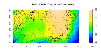
The bei dataset is a point map that shows locations of Beilschmiedia pendula Lauraceae trees (a total of 3604 trees) observed in a 1000 m by 500 m rectangular window. In addition to the point map, a map of elevation and slope gradient is provided in the bea.extra dataset:
> str(bei.extra, max.level=1)
> plot(bei.extra$elev, main="Beilschmiedia pendula Lauraceae")
> plot(bei, add=TRUE, pch=16, cex=0.3)
We can extend this initial list of covariates and attach two more maps: the wetness index and vertical distance from the channel network (derive in SAGA and import back to R):
> grids <- as(bei.extra[[1]], "SpatialGridDataFrame")
> names(grids)[1] <- "elev"
> grids$grad <- as(bei.extra[[2]], "SpatialGridDataFrame")$v
> write.asciigrid(grids["elev"], "dem.asc")
> # Generate the wetness index and vertical distance from the channel network:
> rsaga.esri.to.sgrd(in.grids="dem.asc", out.sgrds="dem.sgrd", in.path=getwd())
> rsaga.geoprocessor(lib="ta_hydrology", module=15, param=list(DEM="dem.sgrd", C="catharea.sgrd",
+    GN="catchslope.sgrd", CS="modcatharea.sgrd", SB="twi.sgrd", T=10))
> rsaga.geoprocessor(lib="ta_channels", module=0, param=list(ELEVATION="dem.sgrd",
+    CHNLNTWRK="chnlntwrk.sgrd", CHNLROUTE="channel_route.sgrd", SHAPES="channels.shp",
+    INIT_GRID="dem.sgrd", DIV_CELLS=5, MINLEN=10))
> rsaga.geoprocessor(lib="ta_channels", module=3, param=list(ELEVATION="dem.sgrd", CHANNELS="chnlntwrk.sgrd",
+    ALTITUDE="achan.sgrd", THRESHOLD=0.1, NOUNDERGROUND=TRUE))
> rsaga.sgrd.to.esri(in.sgrds=c("twi.sgrd","achan.sgrd"), out.grids=c("twi.asc","achan.asc"), prec=1, out.path=getwd())
> grids$achan <- readGDAL("achan.asc")$band1
> grids$twi <- readGDAL("twi.asc")$band1
Kernel density estimation
Before we run kernel smoothing, we can try estimating the optimal bandwidth size; using the method of Berman and Diggle (1989):
> gridbbox <- as.points(list(x=c(grids@bbox[1,1],grids@bbox[1,2],grids@bbox[1,2],grids@bbox[1,1]),
+     y=c(grids@bbox[2,1],grids@bbox[2,1],grids@bbox[2,2],grids@bbox[2,2])))
> mserw <- mse2d(as.points(coordinates(bei.pnt)), gridbbox, 100, 10*bei.pixsize)
> bw <- mserw$h[which.min(mserw$mse)]
> plot(mserw$h,mserw$mse, type="l")
This shows that the optimal bandwidth size is about 4 m. But since our grid cell size is 5 m, this bandwidth is not really suited for this scale of work. Based on the plot from above, we only know that we should not use a bandwidth smaller than 5 m, higher bandwidths are all plausible.
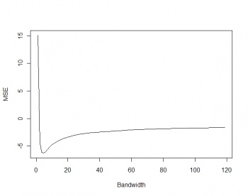 Figure: Selection of the optimal bandwidth using the method of Berman and Diggle (1989). |
We also consider the least squares cross validation method to select the bandwidth size using the method of Worton (1995), and as implemented in the adehabitat package:
> bei.pnt <- data.frame(x=bei$x, y=bei$y, no=rep(1, length(bei$x)))
> coordinates(bei.pnt) <- ~x+y
> dem.asc <- import.asc("dem.asc")
> bei.kdens <- kernelUD(xy=as.data.frame(bei.pnt@coords), id=NULL, h="LSCV", grid=dem.asc)
Warning message:
In kernelUD(xy = as.data.frame(bei.pnt@coords), id = NULL, h = "LSCV",  :
  The algorithm did not converge
within the specified range of hlim: try to increase it
This does not converge, hence we need to set the bandwidth size using some ad hoc method (this is unfortunately a very common problem with many real point patterns) e.g.:
bei.pixsize <- sqrt(areaSpatialGrid(grids)/length(bei$x))
bei.pixsize
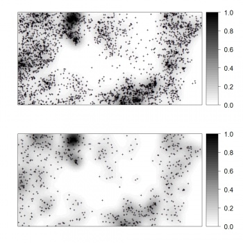
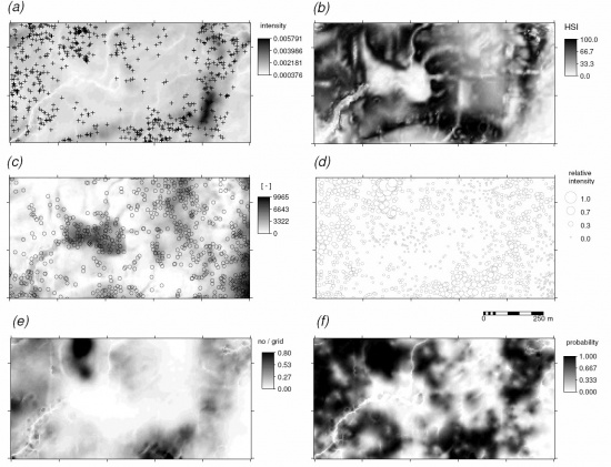
We next derive a relative kernel intensity map (shown below):
> bei.dens <- density(bei.ppp, sigma=2*bei.pixsize)
> grids$dens <- as(bei.dens, "SpatialGridDataFrame")$v
> grids$densr <- grids$dens/(max(grids$dens, na.rm=T))
> bei.pnt.plot <- list("sp.points", bei.pnt, pch="+", cex=.7, col="black")
> plt.dens1 <- spplot(grids["densr"], scales=list(draw=F), at=seq(0,1,0.025),
+      col.regions=grey(rev(seq(0,1,0.025))), sp.layout=bei.pnt.plot)
If we randomly subset the original occurrence locations and then re-calculate the relative density, we can notice that the spatial pattern of the two maps does not really differ, neither do their histograms differ. This supports our assumption that the relative density map can be indeed reproduced from a representative sample.
> bei.pnt$rnd <- runif(length(bei.pnt$no))
> bei.sub.pnt <- subset(bei.pnt, bei.pnt$rnd<0.2)
> bei.sub <- bei
> bei.sub$x <- coordinates(bei.sub.pnt)[,1]
> bei.sub$y <- coordinates(bei.sub.pnt)[,2]
> bei.sub$n <- length(coordinates(bei.sub.pnt)[,2])
> bei.sub.dens <- density(bei.sub, sigma=2*bei.pixsize)
> grids$sub.dens <- as(bei.sub.dens, "SpatialGridDataFrame")$v
> grids$sub.densr <- grids$sub.dens/(max(grids$sub.dens, na.rm=T))
> bei.sub.pnt.plot <- list("sp.points", bei.sub.pnt, pch="+", cex=.7, col="black")
> plt.dens2 <- spplot(grids["sub.densr"], scales=list(draw=F), at=seq(0,1,0.025),
+      col.regions=grey(rev(seq(0,1,0.025))), sp.layout=bei.sub.pnt.plot)
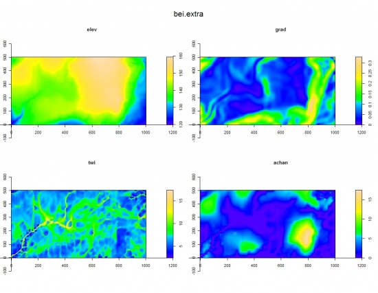
We proceed with how much are the environmental predictors correlated with the intensity values. We can extend the original single auxiliary map (elev) by adding some hydrological parameters: slope, topographic wetness index and altitude above channel network.
> bei.extra$twi <- as.im(as.image.SpatialGridDataFrame(grids["twi"]))
> bei.extra$achan <- as.im(as.image.SpatialGridDataFrame(grids["achan"]))
> plot(bei.extra)
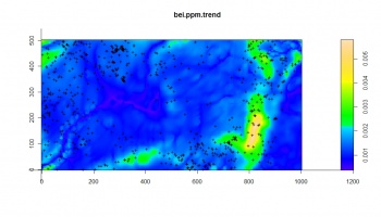
The result of fitting a non-stationary point process with a loglinear intensity using the ppm method of spatstat shows that intensity is negatively correlated with wetness index, and positively correlated with all other predictors.
> bei.sub.ppm <- ppm(bei.sub, ~elev+grad+twi+achan, covariates=list(elev=bei.extra$elev,
+     grad=bei.extra$grad, twi=bei.extra$twi, achan=bei.extra$achan))
> summary(bei.sub.ppm)
Point process model
fitted by maximum pseudolikelihood (Berman-Turner approximation)
Call:
ppm(Q = bei.sub, trend = ~elev + grad + twi + achan, covariates = list(elev = bei.extra$elev,...
Edge correction: “border”
----------------------------------------------------
FITTED MODEL:

Nonstationary Poisson process

 ---- Intensity: ----

Trend formula: ~elev + grad + twi + achan
Model involves external covariates

Fitted coefficients for trend formula:
(Intercept)        elev        grad         twi       achan
-9.00309481  0.01675857  4.24494406 -0.07240637  0.03017035

> bei.ppm.trend <- predict(bei.sub.ppm, type="trend",
+     ngrid=c(grids@[email protected][2],grids@[email protected][1]), window=as(grids[1], "owin"))
> plot(bei.ppm.trend)
> plot(bei.sub, add=T, pch=".")
A comparison between the Akaike Information Criterion (AIC) for a model without predictors and with predictors shows that there is a slight gain in using the covariates to predict the intensity. Visually, we can see that the predicted trend seriously misses some hot-spots/clusters of points. This demonstrates that using only point pattern analysis techniques to map species' distribution with covariates will be of limited use.
> fitnull <- ppm(bei.sub, ~1)
> AIC(fitnull)
> AIC(bei.sub.ppm) # this is a slightly better model
> bei.sub.ppm.step <- step(bei.sub.ppm)
# all four predictors are significant
Habitat Suitability Analysis
We proceed with the Environmental-Niche Factor Analysis (Hirzel et al. 2002), as implemented in the adehabitat package (Calenge, 2006):
> beidata <- data2enfa(as.kasc(list(dem=import.asc("dem.asc"), grad=import.asc("grad.asc"),
+     twi=import.asc("twi.asc"), achan=import.asc("achan.asc"))), bei.sub.pnt@coords)
# run ENFA and make predictions of habitat suitability index:
> enfa.bei <- enfa(dudi.pca(beidata$tab, scannf=FALSE), beidata$pr, scannf=FALSE, nf=2)
> bei.dist <- predict(enfa.bei, beidata$index, beidata$attr)
# image(bei.dist)
> grids$bei.dist <- as.SpatialGridDataFrame.im(asc2im(bei.dist))$v
> sum.dist <- summary(grids$bei.dist)
> grids$rankv <- rank(grids$bei.dist, ties.method="first")
> grids$hsit <- ifelse(grids$bei.dist<sum.dist[["Median"]], (1-grids$rankv/max(grids$rankv))*100,
+    (1-grids$rankv/max(grids$rankv))*100)
> grids$hsi <- 100*round((grids$hsit-min(grids$hsit, na.rm=T))/(max(grids$hsit,
+     na.rm=T)-min(grids$hsit, na.rm=T)), 3)
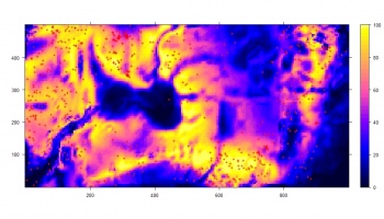
> plt.HSI <- spplot(grids["hsi"], at=seq(0,100,2.5), col.regions=bpy.colors())
It shows that this species generally avoids the areas of high wetness index, i.e. it prefers ridges/dry positions. This spatial correlation is now more distinct (compare with the trend model in the figure above). This demonstrates the power of ENFA, which is in this case more suited for analysis of the occurrence-only locations than the regression analysis or the point pattern analysis.
Simulation of pseudo-absences
The pseudo-absences (which we will use further for regression modelling) can be simulated using the HSI and the distance to observation points as the weight maps:
# first the buffer distance:
> rsaga.geoprocessor(lib="grid_gridding", module=3, param=list(GRID="bei_buffer.sgrd",
+    INPUT="bei_sub.shp", FIELD=0, LINE_TYPE=0, USER_CELL_SIZE=grids@grid@cellsize[[1]],
+    USER_X_EXTENT_MIN=grids@bbox[1,1]+grids@grid@cellsize[[1]]/2,
+    USER_X_EXTENT_MAX=grids@bbox[1,2]-grids@grid@cellsize[[1]]/2,
+    USER_Y_EXTENT_MIN=grids@bbox[2,1]+grids@grid@cellsize[[1]]/2,
+    USER_Y_EXTENT_MAX=grids@bbox[2,2]-grids@grid@cellsize[[1]]/2))
# now extract a buffer distance map and load it back to R:
# the parameters DIST and IVAL are estimated based on the grid properties:
> rsaga.geoprocessor(lib="grid_tools", module=10, param=list(SOURCE="bei_buffer.sgrd",
+   DISTANCE="bei_dist.sgrd", ALLOC="bei_alloc.sgrd", BUFFER="bei_bdist.sgrd",
+   DIST=sqrt(areaSpatialGrid(grids))/3, IVAL=grids@grid@cellsize[[1]]))
> rsaga.sgrd.to.esri(in.sgrds="bei_dist.sgrd", out.grids="bei_dist.asc",
+   out.path=getwd(), prec=1)

> grids$buffer <- readGDAL("bei_dist.asc")$band1
> grids$bufferr <- grids$buffer/max(grids$buffer, na.rm=T)
# extrapolation weight:
> grids$weight <- ((100*grids$bufferr+(100-grids$hsi))/2)^2
> dens.weight <- as.im(as.image.SpatialGridDataFrame(grids["weight"]))
> bei.absences <- rpoint(length(bei.sub.pnt$no), f=dens.weight)
> bei.absences <- data.frame(x=bei.absences$x, y=bei.absences$y ,no=rep(0,
+    length(bei.sub.pnt$no)))
> coordinates(bei.absences) <- ~x+y
# combine the occurences and absences:
> bei.all <- rbind(bei.sub.pnt["no"], bei.absences["no"])
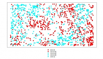
> spplot(bei.all["no"], col.regions=rainbow(2), cex=1.2)
By combining HSI and buffer map around the occurrence locations, we are able to simulate the same amount of pseudo-absence locations. Note that the correlation between the HSI and intensity is now clearer, and the spreading of the points around the HSI feature space is symmetric.
Regression analysis / variograms
Before we run any regression analysis, we need to derive principal components using the four environmental predictors (in order to reduce their dimensions and multicolinearity):
# derive PCs from the original predictors:
> pc.grids <- prcomp(~grad+elev+twi+achan, scale=TRUE, grids)
> pc.comps <- as.data.frame(pc.grids$x)
> pointgrids <- as(grids, "SpatialPointsDataFrame")
> pc.comps$X <- coordinates(pointgrids)[,1]
> pc.comps$Y <- coordinates(pointgrids)[,2]
> coordinates(pc.comps) <- ~X+Y
> gridded(pc.comps) <- TRUE
> pc.comps <- as(pc.comps, "SpatialGridDataFrame")
Next, we can overlay the predictors and the estimated intensities at occurrence and absence locations:
> bei.ov2 <- overlay(pc.comps, bei.all)
> bei.ov2$no <- bei.all$no
# convert the original values to logits:
> bei.ov2$log.densr <- log((bei.ov2$densr+0.001)/(1-(bei.ov2$densr-0.001)))
> summary(bei.ov2$log.densr); var(bei.ov2$log.densr, na.rm=T)
   Min. 1st Qu.  Median    Mean 3rd Qu.    Max.
 -6.908  -3.378  -1.882  -2.297  -1.197   4.253
[1] 3.666165
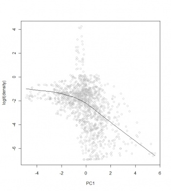
The benefit of converting the target variable to logits and the predictors to PCs, is that the relationship between the two is now close to linear:
> scatter.smooth(bei.ov2$PC1, bei.ov2$log.densr, span=19/20, col="grey",
+    xlab="PC1", ylab="logit(density)")
> lm3.bei <- lm(log.densr~PC1+PC2+PC3+PC4, bei.ov2@data)
> summary(lm3.bei)
# the model explains 24 % of variation
The model fitting is more successful after insertion of the pseudo-absences: the adjusted R-square fitted using the four environmental predictors jumped from 0.07 to 0.28. This demonstrates the benefits of inserting the pseudo-absence locations. If we would randomly insert the pseudo-absences, the model would not improve (or would become even noisier).
To fit a GLM with a binomial model you can use:
glm.bei <- glm(no~PC1+PC2+PC3+PC4, bei.ov2@data, family=binomial())
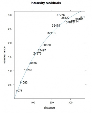
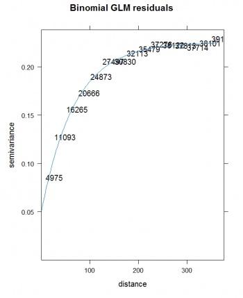
We can now deal with the residuals by using some standard geostatistical techniques (Pebesma et al. 2005). To fit a variogram for the residuals, we use the gstat package:
> res.var <- variogram(residuals(lm3.bei)~1, bei.ov2)
> res.vgm <- fit.variogram(res.var, vgm(nugget=0, model="Exp", range=sqrt(areaSpatialGrid(grids))/3,
+    psill=var(residuals(lm3.bei), na.rm=T)))
plot(res.var, res.vgm, plot.nu=T, pch="+", main="Intensity residuals")
Final predictions
We can finally generate predictions using a regression-kriging model (gstat package):
# regression part:
> vt.gt <- gstat(id=c("dens"), formula=log.densr~PC1+PC2+PC3+PC4, data=bei.ov2)
# residuals:
> vt.gr <- gstat(id=c("dens"), formula=residuals(lm3.bei)~1, data=bei.ov2, model=res.vgm)
> vt.reg <- predict.gstat(vt.gt, pc.comps) # regression part
> vt.ok <- predict.gstat(vt.gr, pc.comps, nmax=80, beta=1, BLUE=FALSE, debug.level=-1)
> vt.reg$dens <- exp(vt.reg$dens.pred+vt.ok$dens.pred)/(1+exp(vt.reg$dens.pred+vt.ok$dens.pred))
> vt.reg$densA <- vt.reg$dens * length(bei.pnt$no)/sum(vt.reg$dens, na.rm=F)
> sum(vt.reg$densA) # check if the sum of counts equals the population!
The resulting map of intensity predicted using regression-kriging is indeed a hybrid map that reflects features from kernel smoothing (hot spots) and environmental patterns, thus it is a map richer in contents than the pure intensity map estimated using kernel smoothing only, or the Habitat Suitability Index. Note also that, although the GLM-kriging with bimodial link function is statistically a more straight forward procedure (it is completely independent from point pattern analysis), it's output is limited in content because it also misses to represent the hot-spots/quantities of individuals.
Important references:
- Baddeley, A., 2008. Analysing spatial point patterns in R. CSIRO, Canberra, Australia.
- Bivand, R., Pebesma, E., Rubio, V., 2008. Applied Spatial Data Analysis with R. Use R Series. Springer, Heidelberg.
- Calenge, C., 2007. Exploring Habitat Selection by Wildlife with adehabitat. Journal of Statistical Software 22(6), 2--19.
- Christensen, R., 2001. Linear Models for Multivariate, Time Series, and Spatial Data. 2nd Edition. Springer Verlag, New York, p. 393.
- Diggle, P.J., 2003. Statistical Analysis of Spatial Point Patterns, 2nd Edition. Arnold Publishers.
- Engler, R., Guisan, A., Rechsteiner, L., 2004. An improved approach for predicting the distribution of rare and endangered species from occurrence and pseudo-absence data. Journal of Applied Ecology 41 (2), 263-274.
- Hirzel A.H., Hausser J., Chessel D. & Perrin N., 2002. Ecological-niche factor analysis: How to compute habitat-suitability maps without absence data? Ecology, 83, 2027-2036.
- Pebesma, E.J., Duin, R.N.M., Burrough, P.A., 2005. Mapping sea bird densities over the North Sea: spatially aggregated estimates and temporal changes. Environmetrics 16(6), 573--587.
- Tsoar, A., Allouche, O., Steinitz, O., Rotem, D., Kadmon, R., 2007. A comparative evaluation of presence-only methods for modelling species distribution. Diversity & Distributions 13(9), 397--405.
<Rating> Rate this article: 1 Poor and in error 2 Far from ready 3 Needs improvements 4 Minor corrections 5 Very useful!! </Rating>
