Interpolation of ISRIC-WISE international soil profile data
SRIC WISE is the international soil profile dataset, a selection of globally distributed soil profiles, prepared by the International Soil Reference and Information Centre (ISRIC) located in Wageningen (Batjes, 2008; 2009). The most recent version (3.1) of the soil profile database contains 10,253 profiles (not all profiles are complete!). The database (as any database) consists of several tables, the most important are: WISE3_SITE (information about the soil profile site) and WISE3_HORIZON (laboratory data per horizon). This article demonstrates how to interpolate some important soil properties using regression-kriging and a large repository of publicly accessible global environmental maps (about 10 km resolution).
The maps presented here were created for demonstration purposes. The true accuracy/consistency of these maps has not been evaluated and is heavily controlled by the representativeness of the sampling pattern and accuracy of individual measurements (refer to the ISRIC WISE general disclaimer). Compare also with the global soil property maps distributed by USGS and/or ISRIC. An updated version of this article can be followed in Hengl (2009; ch.7).
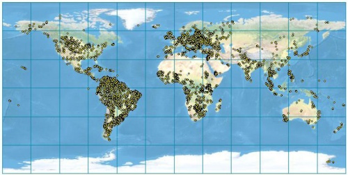 Figure: Global distribution of soil profiles in the ISRIC WISE v3 database. After Batjes (2008). |
To run this script, you first need to obtain the MS Access file from the ISRIC website. Before you start using ISRIC WISE database, please also read about its limitations. You will also need to obtain and install the necessary software: R (including RSAGA, RODBC, maptools and gstat packages) and SAGA GIS. If you require more help with understanding the R syntax, consider following some of the R on-line guides.
|
Contents |
Loading the data
First, download and unzip all relevant predictors from the web-repository. This takes few steps:
# location of maps:
> URL <- "http://spatial-analyst.net/worldmaps/"
# list of maps:
> map.list <- c("biocl01", "biocl02", "biocl04", "biocl05", "biocl06", "biocl12", "biocl15", "countries", "dcoast",
+     "globedem", "landcov", "landmask", "nlights", "pcndvi1", "pcndvi2", "pcndvi3", "pcpopd1", "himpact",
+     "glwd31", "wildness", "wwfeco", "soiltype", "quakein", "iflworld", "chlo08", "chlo08s")
# download the zipped maps one by one:
> for(i in 1:length(map.list)) {
>  download.file(paste(URL, map.list[i], ".zip", sep=""),
  +   destfile=paste(getwd(), "/", map.list[i], ".zip", sep=""))
>  fname <- zip.file.extract(file=paste(map.list[i], ".asc", sep=""),
  +    zipname=paste(map.list[i], ".zip", sep=""))
>  file.copy(fname, paste("./", map.list[i], ".asc", sep=""), overwrite=TRUE)
>  fname <- zip.file.extract(file=paste(map.list[i], ".rdc", sep=""),
  +   zipname=paste(map.list[i], ".zip", sep=""))
>  file.copy(fname, paste("./", map.list[i], ".rdc", sep=""), overwrite=TRUE)
# Delete the zip files:
>  unlink(paste(map.list[i], ".zip", sep=""))
> }
If this was successful, you will notice that the ArcInfo ASCII grids are now available in your working directory.
Second, you need to obtain the ISRIC-WISE_ver3.mdb file, to which you can then connect by using the RODBC package:
> cGSPD <- odbcConnectAccess("ISRIC-WISE_ver3.mdb")
# Look at available tables:
> sqlTables(cGSPD)$TABLE_NAME
 [1] "MSysAccessObjects"
 [2] "MSysAccessXML"
 [3] "MSysACEs"
 [4] "MSysObjects"
 [5] "MSysQueries"
 [6] "MSysRelationships"
 [7] "WISE3__ReadMeFirst"
 [8] "WISE3_coding_conventions"
 [9] "WISE3_HORIZON"
[10] "WISE3_LABcodes_Description"
[11] "WISE3_LABname"
[12] "WISE3_LABname_codes"
[13] "WISE3_SITE"
[14] "WISE3_SOURCE"
Now that we have connected to the database, we can prepare a point map with soil attributes of interest. We are interested in the following five variables:
- ORGC = Organic carbon content (promille or g C kg-1);
- SAND, SILT, CLAY = Sand, Silt and Clay content in %;
- TOPDEP, BOTDEP = Thickness of soil horizons in cm;
Because we will generate maps of soil organic carbon and texture fractions for the whole soil profile, we will also collect the depths to which horizons refer:
> GSPD.HOR <- sqlQuery(cGSPD, query="SELECT WISE3_ID, HONU, ORGC, TOPDEP,
+     BOTDEP FROM WISE3_HORIZON")
> str(GSPD.HOR)
'data.frame':   47833 obs. of  8 variables:
 $ WISE3_ID: Factor w/ 10253 levels "AF0001","AF0002",..: 1 1 1 2 2 2 2 3 3 3 ...
 $ HONU    : int  1 2 3 1 2 3 4 1 2 3 ...
 $ ORGC    : num  7.6 2.3 0.9 12.8 6 3.9 2.7 5.9 2.4 NA ...
 $ SAND    : int  40 10 10 40 15 10 40 40 65 60 ...
 $ SILT    : int  40 55 55 40 65 55 40 40 25 15 ...
 $ CLAY    : int  20 35 35 20 20 35 20 20 10 25 ...
 $ TOPDEP  : int  0 15 60 0 20 60 110 0 20 50 ...
 $ BOTDEP  : int  15 60 150 20 60 110 170 20 50 110 ...
where HONU is the horizon number (from the soil surface) and TOPDEP and BOTDEP are the upper and lower horizon depths. This shows that there are over 45 thousand measurements of the four variables of interest. The number of soil profiles is in fact much smaller -- as you can see from the WISE3_ID column, there are 10,253 unique IDs/profiles in total.
Because we are interested in the cumulative values of the target variables, we need to aggregate them per profile. For example, to estimate the mean organic carbon content for the soil profile, we need to divide the measured values of ORGC with the thickness of horizon:
> GSPD.HOR$HOTH <- GSPD.HOR$BOTDEP-GSPD.HOR$TOPDEP
> GSPD.HOR$ORGC.d <- GSPD.HOR$ORGC/GSPD.HOR$HOTH*100  # g kg-1 m-1;
> summary(GSPD.HOR$ORGC.d)
       Min.     1st Qu.      Median
    0.03226     8.40000    23.33000
       Mean     3rd Qu.        Max.
  117.50000    70.00000 34100.00000
       NA's
 6256.00000
> GSPD.HOR$SAND.d <- GSPD.HOR$SAND/GSPD.HOR$HOTH*100
> GSPD.HOR$SILT.d <- GSPD.HOR$SILT/GSPD.HOR$HOTH*100
> GSPD.HOR$CLAY.d <- GSPD.HOR$CLAY/GSPD.HOR$HOTH*100
We can now estimate the mean ORGC for the whole profile:
# select only horizons with ORGC!
> GSPD.orgc <- subset(GSPD.HOR, !is.na(GSPD.HOR$ORGC.d)|GSPD.HOR$ORGC.d>0,
+     c("WISE3_ID", "ORGC.d"))
# aggregate OGRC values per profiles:
> GSPD.orgc <- aggregate(GSPD.orgc["ORGC.d"], by=list(GSPD.orgc$WISE3_ID),
+     FUN=mean)
# thickness of soil with biological activity
> GSPD.hoth <- subset(GSPD.HOR, !is.na(GSPD.HOR$ORGC.d)|GSPD.HOR$ORGC.d>0,
+     c("WISE3_ID", "HOTH"))
# aggregate HOTH values to get the thickness of soil:
> GSPD.orgc$HOTH <- aggregate(GSPD.hoth["HOTH"], by=list(GSPD.hoth$WISE3_ID),
+     FUN=sum)$HOTH
which gives the following result:
> GSPD.orgc[1:10,]
   Group.1    ORGC.d HOTH
1   AF0001  18.92593  150
2   AF0002  22.82500  170
3   AF0003  18.75000   50
4   AF0004  69.66667   35
5   AF0005  19.93220  190
6   AL0001  36.37500   94
7   AL0002  35.94204   87
8   AL0003  30.56151   85
9   AL0004 125.91518  120
10  AL0005  22.03333  170
This shows that, for example, the profile "AF0001" has 18.9 g C kg-1 m-1 of soil profile, and is 150 cm thick.
We do the same thing also for the textures:
> GSPD.text <- aggregate(GSPD.HOR[c("SAND.d", "SILT.d", "CLAY.d")],
+    by=list(GSPD.HOR$WISE3_ID), FUN=sum)
> GSPD.text$SUM <- GSPD.text$SAND.d + GSPD.text$SILT.d + GSPD.text$CLAY.d
# back to 100% scale:
> GSPD.text$SAND.d <- GSPD.text$SAND.d/GSPD.text$SUM*100
> GSPD.text$SILT.d <- GSPD.text$SILT.d/GSPD.text$SUM*100
> GSPD.text$CLAY.d <- GSPD.text$CLAY.d/GSPD.text$SUM*100
# replace zero/100% values
> GSPD.text$SAND.d <- ifelse(GSPD.text$SAND.d==0, 0.5, ifelse(GSPD.text$SAND.d==1,
+    99.5, GSPD.text$SAND.d))
> GSPD.text$SILT.d <- ifelse(GSPD.text$SILT.d==0, 0.5, ifelse(GSPD.text$SILT.d==1,
+    99.5, GSPD.text$SILT.d))
> GSPD.text$CLAY.d <- ifelse(GSPD.text$CLAY.d==0, 0.5, ifelse(GSPD.text$CLAY.d==1,
+    99.5, GSPD.text$CLAY.d))
and combine the two tables:
> GSPD.HORa <- merge(x=GSPD.orgc, y=GSPD.text, all.y=T, all.x=T, by="Group.1")
Next, we want to obtain the coordinates of profiles:
# coordinates of points
> GSPD.latlon <- sqlQuery(cGSPD, query="SELECT WISE3_id, LATIT, LATDEG, LATMIN,
+     LATSEC, LONGI, LONDEG, LONMIN, LONSEC FROM WISE3_SITE")
These need to be converted to arcdegrees. First, we filter the missing coordinates and then convert the multiple columns to a single column:
# make coordinates in arcdegrees:
> GSPD.latlon <- subset(GSPD.latlon, !is.na(GSPD.latlon$LATDEG)&!is.na(GSPD.latlon$LONDEG)&!is.na(GSPD.latlon$LATMIN)&!is.na(GSPD.latlon$LONMIN))
> GSPD.latlon$LATSEC <- ifelse(is.na(GSPD.latlon$LATSEC), 0, GSPD.latlon$LATSEC)
> GSPD.latlon$LONSEC <- ifelse(is.na(GSPD.latlon$LONSEC), 0, GSPD.latlon$LONSEC)
# define a new function to merge the degree, min, sec columns:
> cols2dms <- function(x,y,z,e){as(char2dms(paste(x, "d", y, "'", z, "\"", e, sep="")), "numeric")}
> GSPD.latlon$LAT <- cols2dms(GSPD.latlon$LATDEG, GSPD.latlon$LATMIN, GSPD.latlon$LATSEC, GSPD.latlon$LATIT)
> GSPD.latlon$LON <- cols2dms(GSPD.latlon$LONDEG, GSPD.latlon$LONMIN, GSPD.latlon$LONSEC, GSPD.latlon$LONGI)
The two table (horizon properties and profile locations) can be merged by using:
> GSPD <- merge(x=data.frame(locid=GSPD.latlon$WISE3_id, LAT=GSPD.latlon$LAT,
+     LON=GSPD.latlon$LON), y=data.frame(locid=GSPD.HORa$Group.1, HOTH=GSPD.HORa$HOTH,
+     ORGC=GSPD.HORa$ORGC.d, SAND=GSPD.HORa$SAND.d, SILT=GSPD.HORa$SILT.d,
+     CLAY=GSPD.HORa$CLAY.d), all.y=F, all.x=T, sort=F, by.x="locid")
> str(GSPD)
'data.frame':   8065 obs. of  8 variables:
 $ locid: Factor w/ 10253 levels "AF0001","AF0002",..: 35 36 37 38 39 40 41 42 43 44 ...
 $ LAT  : num  40.7 40.7 41.1 41.7 40.6 ...
 $ LON  : num  20.8 19.7 20.6 19.7 19.5 ...
 $ HOTH : int  170 110 163 160 126 180 258 140 143 275 ...
 $ ORGC : num  18 16 37 168.2 39.7 ...
 $ SAND : num  31.18 10.18 9.07 2.12 18.07 ...
 $ SILT : num  35.3 64.8 32.7 39.3 67.5 ...
 $ CLAY : num  33.5 25.1 58.3 58.6 14.4 ...
which can be converted to a point map and exported to a shape file:
> coordinates(GSPD) <-~LON+LAT
> proj4string(GSPD) <- CRS("+proj=longlat +ellps=WGS84")
> writeOGR(GSPD, "GSPD.shp", "ORGC", "ESRI Shapefile")
Because we will use SAGA GIS to run interpolation, you will also need to convert the downloaded worldmaps to SAGA grid format:
> rsaga.esri.to.sgrd(in.grids=set.file.extension(map.list, ".asc"),
+    out.sgrds=set.file.extension(map.list, ".sgrd"), in.path=getwd())
Regression modeling
Now that we have prepared a point map representing showing values of aggregated target variables, we can overlay the points over predictors (worldmaps) and prepare a regression matrix. Because the amount of maps is large, we run this operation in SAGA:
> rsaga.geoprocessor(lib="shapes_grid", module=0, param=list(SHAPES="GSPD.shp",
+     GRIDS=paste(set.file.extension(map.list, ".sgrd"), collapse=";"),
+     RESULT="GSPD_ov.shp", INTERPOL=0))  # simple overlay
This will produce a point shape file, which we can then read back to R:
> GSPD.ov <- readShapePoints("GSPD_ov.shp", CRS("+proj=longlat +ellps=WGS84"))
# fix the names:
> names(GSPD.ov@data)[7:length(GSPD.ov@data)] <- map.list
> str(GSPD.ov@data)
'data.frame':   8065 obs. of  32 variables:
 $ LOCID    : Factor w/ 8065 levels "AF0001","AF0002",..: 35 36 37 38 39 40 41 42 43 44 ...
 $ HOTH     : num  170 110 163 160 126 180 258 140 143 275 ...
 $ ORGC     : num  18 16 37 168.2 39.7 ...
 $ SAND     : num  31.18 10.18 9.07 2.12 18.07 ...
 $ SILT     : num  35.3 64.8 32.7 39.3 67.5 ...
 $ CLAY     : num  33.5 25.1 58.3 58.6 14.4 ...
 $ biocl01  : num  91 157 106 148 163 106 54 107 74 56 ...
 $ biocl02  : num  91 157 106 148 163 106 54 107 74 56 ...
 $ biocl04  : num  6515 5768 6443 6420 5430 ...
 $ biocl05  : num  254 294 264 293 292 264 231 311 242 226 ...
 $ biocl06  : num  -40 42 -22 24 56 -22 -105 -78 -77 -96 ...
 $ biocl12  : num  847 1018 899 1402 968 ...
 $ biocl15  : num  30 46 30 43 54 30 48 42 49 50 ...
 $ countries: num  2 2 2 2 2 2 11 11 11 11 ...
 $ dcoast   : num  119 40 102 7 12 102 329 327 325 322 ...
 $ globedem : num  1310 26 686 2 4 ...
 $ landcov  : num  4 11 11 1 11 11 11 10 11 11 ...
 $ landmask : num  1 1 1 1 1 1 1 1 1 1 ...
 $ nlights  : num  0 6 0 8 6 0 4 22 0 0 ...
 $ pcndvi1  : num  2767 2682 2701 2749 2717 ...
 $ pcndvi2  : num  8 -185 -88 -108 -194 -88 150 15 117 156 ...
 $ pcndvi3  : num  100 145 65 112 140 65 134 74 66 61 ...
 $ pcpopd1  : num  198 468 243 335 393 ...
 $ himpact  : num  1 1 0 0 1 0 1 1 1 1 ...
 $ glwd31   : num  0 0 1 0 0 1 0 0 0 0 ...
 $ wildness : num  0 0 0 0 0 0 0 0 0 0 ...
 $ wwfeco   : num  297 484 297 484 484 297 415 415 512 512 ...
 $ soiltype : num  99 83 -1 98 98 -1 74 74 92 92 ...
 $ quakein  : num  51.2 73.4 50.2 48.7 68.3 ...
 $ iflworld : num  0 0 0 0 0 0 0 0 0 0 ...
 $ chlo08   : num  -1 -1 3.26 -1 -1 ...
 $ chlo08s  : num  -1 -1 0.09 -1 -1 0.09 -1 -1 -1 -1 ...
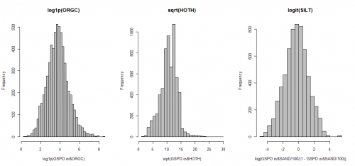
Before we proceed with regression analysis, it is a good idea to visualize histograms for target variables, in order to see if they need to be transformed before the model fitting (close-to-normal distribution is a prerequisite for regression modeling!). You will soon notice that both ORGC and HOTH need to be transformed before regression modeling. In addition, we know that the texture variables (SAND, SILT, CLAY) need to be transformed using the logit transformation to avoid predicting values <0 or >100%.
We can now fit a regression model e.g.:
> orgc.formula <- as.formula(paste("log1p(ORGC)~", paste(sub(".asc", "",
+    map.list[-c(8,12,21,25,26)]), collapse="+")))  # some maps we do not need!
> orgc.formula
log1p(ORGC) ~ biocl01 + biocl02 + biocl04 + biocl05 + biocl06 +
    biocl12 + biocl15 + dcoast + globedem + landcov + nlights +
    pcndvi1 + pcndvi2 + pcndvi3 + pcpopd1 + himpact + glwd31 +
    wildness + soiltype + quakein + iflworld
> lm.ORGC <- lm(orgc.formula, GSPD.ov@data)
> slm.ORGC <- step(lm.ORGC, trace=-1) # step-wise regression
> summary(slm.ORGC)$adj.r.squared
[1] 0.3696821
# 37% of variability!
This shows that the predictors explain 38% of variability in the ORGC values (average density of organic carbon in the soil). For Digital Soil Mapping projects (Lagacherie et al. 2006), this is a significant value.
For practical reasons (computational intensity), we will focus on the top20 predictors only. These can be selected by using:
> attr(summary(slm.ORGC)$coefficients[rank(summary(slm.ORGC)$coefficients[,4])<20,1], "names")[-1]
 [1] "biocl01"    "biocl06"
 [3] "biocl12"    "landcov13"
 [5] "pcndvi3"    "himpact"
 [7] "glwd314"    "glwd3111"
 [9] "wildness"   "soiltype1"
[11] "soiltype6"  "soiltype33"
[13] "soiltype54" "soiltype60"
[15] "soiltype80" "soiltype81"
[17] "soiltype82" "soiltype97"
This process can be automated for each variable of interest:
> lm.formula <- as.list(rep(NA, 5))
> lm.formula[[1]] <- as.formula(paste("log1p(ORGC)~", paste(sub(".asc", "",
+      map.list[-c(8,12,21,25,26)]), collapse="+")))
...
> lm.formula[[5]] <- as.formula(paste("log(CLAY/100/(1-CLAY/100))~",
+      paste(sub(".asc", "", map.list[-c(8,12,21,25,26)]), collapse="+")))
After we have determined 20 significant predictors for all variables of interest, we can make predictions for target variables by using the SAGA multiple linear regression module. Before we can run the predictions in SAGA, we need to prepare the indicator maps and the point map that with transformed variables, e.g. to prepare indicators for different classes of land cover, we can use:
> for(j in c("2","7","8","9","8","12")){
>  worldmaps$tmp <- ifelse(worldmaps$landcov==j, 1, 0)
>  write.asciigrid(worldmaps["tmp"], paste("landcov", j, ".asc", sep=""),
+     na.value=-1)
> }
We also need to prepare the point map with transformed target variables:
> GSPD.ov$ORGC.t <- log1p(GSPD.ov$ORGC)
> GSPD.ov$HOTH.t <- sqrt(GSPD.ov$HOTH)
> GSPD.ov$SAND.t <- log(GSPD.ov$SAND/100/(1-GSPD.ov$SAND/100))
> GSPD.ov$SILT.t <- log(GSPD.ov$SILT/100/(1-GSPD.ov$SILT/100))
> GSPD.ov$CLAY.t <- log(GSPD.ov$CLAY/100/(1-GSPD.ov$CLAY/100))

> target.list <- c("ORGC.t","HOTH.t","SAND.t","SILT.t","CLAY.t")
> writeOGR(GSPD.ov[target.list], "GSPD_ov.shp", "GSPD_ov", "ESRI Shapefile")
Now we can use SAGA GIS to run multiple linear regression (in a loop):
for(i in 1:length(lm.formula)) {
> rsaga.geoprocessor(lib="geostatistics_grid", module=4,
+    param=list(GRIDS=paste(set.file.extension(predictors.list[[i]], ".sgrd"),
+    collapse=";"), SHAPES="GSPD_ov.shp", ATTRIBUTE=i-1, TABLE="regout.dbf",
+    RESIDUAL=set.file.extension(paste("res_", target.list[i], sep=""), ".shp"),
+    REGRESSION=set.file.extension(paste("reg_", target.list[i], sep=""), ".sgrd"),
+    INTERPOL=0))
> }
Modeling spatial auto-correlation
To fit the variograms, we need to first derive the residuals:
> for(i in 1:length(lm.formula)) {
> rsaga.sgrd.to.esri(in.sgrds=set.file.extension(paste("reg_", target.list[i],
+     sep=""), ".sgrd"), out.grids=set.file.extension(paste("reg_", target.list[i],
+     sep=""), ".asc"), out.path=getwd(), pre=3)
> worldmaps@data[paste("reg_", target.list[i], sep="")] <-
+     readGDAL(set.file.extension(paste("reg_", target.list[i], sep=""),
+     ".asc"))$band1
> tmp <- overlay(worldmaps[paste("reg_", target.list[i], sep="")], GSPD.ov)
> GSPD.ov@data[paste("res_", target.list[i], sep="")] <-
+     GSPD.ov@data[target.list[i]]-tmp@data[paste("reg_", target.list[i], sep="")]
> }
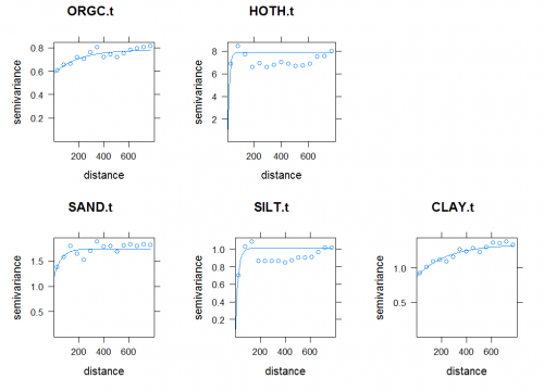
This will read predicted values from the multiple linear regression (from SAGA to R), overlay the original point data and then estimate the residuals. The variograms can now be fitted using:
> vgm.list <- as.list(rep(NA, length(lm.formula)))
> plotvgm.list <- as.list(rep(NA, length(lm.formula)))
> for(i in 1:length(lm.formula)) {
> sel <- !is.na(GSPD.ov@data[paste("res_", target.list[i], sep="")])[,1]
> tmp <- variogram(as.formula(paste("res_", target.list[i], "~1", sep="")),
+      GSPD.ov[sel,], cutoff=800)
> vgm.list[[i]] <- fit.variogram(tmp, vgm(nugget=var(GSPD.ov@data[paste("res_",
+      target.list[i], sep="")], na.rm=T)[1]/3, model="Exp", range=800,
+      sill=var(GSPD.ov@data[paste("res_", target.list[i], sep="")], na.rm=T)[1]))
> plotvgm.list[[i]] <- plot(tmp, vgm.list[[i]], main=target.list[i])
> }
All variograms show relatively high nuggets. The question remains whether the models would improve if one would consider fitting variogram models locally, or by using finer-grain predictors (<10 km) that are maybe able to explain short-range variation.
Final predictions and summary points
Once we have interpolated both thickness of soil profile (HOTH) and the mean organic carbon content (ORGC), we can estimate the total organic carbon in kg C m-2:
where 1682 kg m-3 is the average soil density (approximate number). It makes sense to model the relative organic carbon content and thickness of soil separately, because one can observe both shallow soils with high and low ORGC content and vice versa (many soils with high ORGC are shallow).
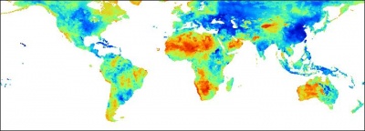 Figure: Predicted sand (%) content in the whole soil profile (0.5 arcdegree grid). |
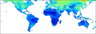 Figure: Predicted silt (%) content in the whole soil profile (0.5 arcdegree grid). |
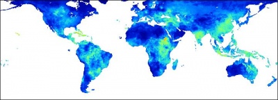 Figure: Predicted clay (%) content in the whole soil profile (0.5 arcdegree grid). |
The gridded predictors used in this exercise explain between 10--40% of variability in the values (38% for ORGC, 11% for HOTH, 22% for SAND, 28% for SILT, 15% for CLAY), which means that these maps are of limited precision. The variograms show relatively high nugget, which also means that about 30--60% of variability in these target variables can not be explained by regression-kriging. Nevertheless, main patterns of soil parameters produced here fit our empirical knowledge: high soil organic carbon mainly reflects the cold and wet temperatures; deep soils reflect the tropical regions and high biomass; texture classes are connected with the land cover, relief and soil mapping units.
The maps presented above can be considered to be especially poor where the density of point samples is low (see the map; most of the former Russian federation, Australia, Canada etc.). The advantage of automating the operations (as in this script) is that these maps can be easily updated once the ISRIC WISE becomes more representative and of higher quality. Due to the data processing automation, many other important soil parameters from the ISRIC WISE database could be interpolated using the same technique.
See also:
- http://www.globalsoilmap.net -- International consortium that aims to make a new digital soil map of the world using state-of-the-art and emerging technologies for soil mapping and predicting soil properties at fine resolution.
- ISRIC WISE Global Soil Profile Database
- http://www.pedometrics.org -- The international research group on pedometrics.
References:
- Batjes, N.H., 2008. ISRIC-WISE Harmonized Global Soil Profile Dataset (Ver. 3.1). Report 2008/02, ISRIC – World Soil Information, Wageningen, p. 59. (with dataset)
- Batjes, N.H., 2009. Harmonized soil profile data for applications at global and continental scales: updates to the WISE database. Soil Use and Management 25, 124-127.
- Hengl, T., 2009. A Practical Guide to Geostatistical Mapping, 2nd Edt. University of Amsterdam, 291 p. ISBN: 978-90-9024981-0
- Lagacherie, P., McBratney, A.B., Voltz, M., (eds) 2006. Digital Soil Mapping: An Introductory Perspective. Developments in Soil Science, Volume 31. Elsevier, Amsterdam. 350pp.
<Rating> Rate this article: 1 Poor and in error 2 Far from ready 3 Needs improvements 4 Minor corrections 5 Very useful!! </Rating>
