Grid size calculator
lthough much has been publish on the impact of pixel size on geographic modelling, grid cell size selection is seldom based on the inherent spatial variability of the data. In fact, in most GIS projects, grid resolution is selected without any scientific justification. In ArcGIS package, for example, the default output cell size is suggested by the system using some trivial rule: in the case the point data is being interpolated in spatial analyst, the system will take the shortest side of the study area and divide by 250 to estimate the cell size. Obviously, such pragmatic rules do not have a sound scientific background in cartography nor in geoinformation science.
|
This motivated me to produce methodological guides to select a suitable grid resolution for output maps and based on the inherent properties of the input data. I tried to relate the choice of grid resolution to the concrete cartographic and statistical concepts, namely scale, processing power, positional accuracy, inspection density, spatial correlation and complexity of terrain. Here you can obtain an R script with processing steps explained in detail. For more details see:
- Hengl T., 2006. Finding the right pixel size. Computers and Geosciences, 32(9): 1283-1298.
Contents |
Examples:
| Screen shot (R+SAGA) showing analysis of the data listed below. To obtain and use R+SAGA, follow these instructions. |
Selection of the cell size based on the GPS positioning accuracy
In this example 100 positioning fixes were recorded using the single-fix GPS positioning method at the control point with a known location (Xt=6535950, Yt=5066581.48). The fluctuation of the GPS readings can be seen in figure. The errors ranged from 0.7 to 23.9 m, average error was 8.5 m with a standard distribution of 5.2 m. The error vectors seems to follow the log-normal distribution. The theoretical distribution gave the 95% probability radius of 19.1 m, while the experimental distribution shows somewhat higher value (20.4). A suitable grid resolution for this case is 34.4 m. If this grid resolution is selected, most (95%) of GPS fixes will fall within the right pixels. This number for example corresponds to the resolution of the Landsat imagery. More accurate positioning method would be needed to locate points within the finer grid resolutions. If we would like to use a GPS positioning with grid resolutions of about 15 m, then we would need to use GPS positioning with averaging (5 minutes per point). Higher positional accuracy (5-20 times) can be achieved by using differential correction or WAAS (Wide Area Augmentation System), which can improve accuracy to less than three meters on average. Such accuracy would be compatible with grid resolutions within the range 2-10 m (SPOT or IKONOS imagery).
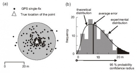 Figure: Selecting the grid resolution based on the confidence radius of the positioning method: (a) 100 single-fix GPS measurements around the true location of the point; (b) histogram of the error vectors, average error vector and the 95% probability confidence radius. After Hengl (2006). |
Selection of the cell size based on the size of agricultural plots
In this example I used an existing polygon map of agricultural fields (figure). The map consists of 121 polygons in total. The smallest polygon is 0.005 ha, the biggest is 6.903 ha, average size of polygons is 0.824 ha with standard deviation of 1.005 ha. The polygons were then separated into two groups according to the shape complexity index. In this case only 6 polygons classified for narrow polygons. For each of these, an average width has been estimated by taking regular measurements (10 per polygon). I further on derived the 5% inverse cumulative distribution value assuming the log-normal distribution. I got 0.046 ha, which means that the pixel size should be about 20 m. The coarsest legible grid size for this data set (P=50%) would be 70 m (A=0.5 ha). If resolutions coarser than 70 m are used to monitor agriculture for this area, then in more than 50% of the areas there will be less than four pixels per polygon. Note that in this case we are not using the true smallest polygon size but somewhat bigger figure (0.046 ha) because the smallest value (0.005 ha) is not representative. The further inspection of the widths showed that the average width of the narrow polygons is about 16 m, which gives a somewhat more strict grid resolution of about 8 m. However, the narrow polygons occupy only 0.9% percents of the the total study area, so we do not have to be as strict. Finally, I would recommend that the satellite imagery in range from 10 to 70 m can be used to monitor agriculture for this study area.
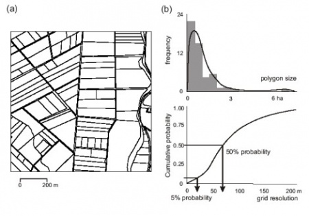 Figure: Selection of the grid resolution based on the average size of the objects observed: (a) agricultural plots; (b) distribution of surfaces for compact plots and related grid resolution. After Hengl (2006). |
Selection of the cell size for interpolation purposes
In this example I will use the Wesepe point data previously used in numerous soil mapping applications (De Gruijter et al., 1997). The dataset consist of 552 profile observations where various soil variables have been described. The target variable is the membership value to enk earth soil type. The values range from 0 to 1, with an average of 0.232 and a standard deviation of 0.322. The total size of the area is 12.1 km^2, which gives a sampling density of about 45 observations per km^2, which corresponds to the scale of 1:25K, i.e. grid resolution of 12 m. If we inspect the spreading of the points, we see that the average spacing between the closest point pairs is about 120 m, which is fairly close to the regular point sampling (for this data set --- 148 m). The cumulative distribution showed that 95% of points are at distances of 5 and more meters. This means that the legible grid resolutions are between 5 and 150 m. Automated fitting of the variogram using a global model further gave a nugget parameter (C0) of 0.042, a sill (C0 + C1) of 0.097 and a range parameter (R) of 175.2 m, which means that the variable is correlated up to the distance of about 525 m (h_R). There are 11807 point pairs within this range, which finally means that the optimal lag/grid size would be about 23 m. The pattern analysis of the point data set further shows that there is clear regularity in the point geometry: most of the distances are grouped at 180 m.
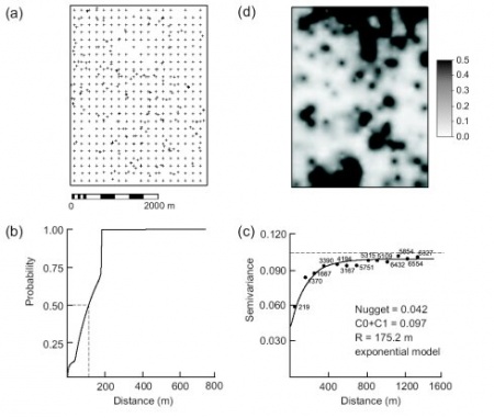 Figure: Selection of grid resolution based on the point pattern analysis: (a) a set of 552 soil profile observations; (b) probability of finding one point in the neighborhood and graph of distances to the closest point; (c) variogram and parameters fitted automatically in gstat, (d) interpolated map using ordinary kriging at grid resolution of 10 m. After Hengl (2006). |
Selection of cell size for geomorphometric analysis
In this case study I will demonstrate how a grid resolution can be selected from a map of contours, i.e. a dataset consisting of lines digitized from a topo-map. Contour lines were extracted from the 1:50K topo-map, with the contour interval of 10 m and supplementary 5 m contours in areas of low relief. The total area is 13.69 km^2 and elevations range from 80 to 240 m. There were 127.6 km of contour lines in total, which means that the average spacing between the contours is 107 m. The grid resolution should be at least 53.5 meters to present the most of the mapped changes in relief. I then derived the distance from the contours map using the 5 m grid and displayed the histogram of the distances to derive the 5% probability distance. Absolutely shortest distance between the contours is 7 meters, and the 5% probability distance is 12.0 m. Finally, I can conclude that the legible resolution for this data set is within range 12.0-53.5 m. Finer resolutions than 12 m are unnecessary for the given complexity of terrain. Note that selection of the most suitable grid resolution based on the contour maps is scale dependant. For the contour lines digitized from the 1:5K topo maps, the average spacing between the lines is 26.6 m and the 5% probability distance is 1.6 m. This means that, at 1:5K scale, the recommended resolutions are between 1.6 and 13.3 m.
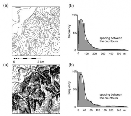 Figure: Selection of the grid resolution based on the complexity of terrain: (a) and (c) contours from the 1:50K and 1:5K topomaps, (b) and (d) histograms of distances between the contours for the two scales. After Hengl (2006). |
Other interesting issues:
1. When does interpolation becomes down-scaling (disaggregation)?
ANSWER: Interpolation becomes down-scaling once the grid resolution in more than 50% of the area is finer than it should be for the given sampling density. For example, in soil mapping, one point sample should cover 160 pixels. If we have 100 samples and the size of the area is 10 km2, then it is valid to map soil variables at resolutions of 25 m (maximum 10 m) or coarser. Note that down-scaling is only valid if we have some auxiliary data (e.g. digital elevation model) which is of finer resolution than the effective grid resolution and which is highly correlated with the variable of interest (in statistics - 'target variable'). In the case from above, to produce maps of resolution of finer than 10 m and without help from significant auxiliary predictors would mean that we are not respecting the soil survey standards.
2. How to select a grid resolution for DEM if the elevation data is collected densely over the area of interest (e.g. GPS height measurements from precision agriculture)?
ANSWER: There are two possibilities. One is to derive a variogram for sampled elevations, then estimate the distance at which are values still auto-correlated (range) and then estimate the bin size following the formula of Izenman (1991). An alternative is to first derive contour lines from the elevation measurements (e. g. in surfer or using the akima package in R). Note that, before deriving the contours, you will have to fit the surface through the measured elevations (e. g. use the splines with tension). This is a sample script to automatically estimate grid cell size using a given point data set (elevations):
UNIQ27156d377dce311b-geshi-00000000-QINU
3. What is a statistically sound approach to select a grid cell size based on the accuracy of DEM-derivatives?
An iterative DEM cell-size optimization algorithm is implemented in the ANUDEM package, following the method of Hutchinson (1996). By plotting the RMS slope versus the grid spacing index, one can select the grid cell size that shows the maximum information content in the slope (relief) map. The optimal grid cell size is the one where further refinement does not change the slope map.
We can implement a similar principle in R, e.g. derive SLOPE maps using several grid cell sizes and then see if they differ significantly. We can start with generating DEMs from point data (e.g. using splines):
UNIQ27156d377dce311b-geshi-00000001-QINU
For each DEM, we derive a SLOPE map:
UNIQ27156d377dce311b-geshi-00000002-QINU
We can now compare the slope maps (whether they differ significantly):
UNIQ27156d377dce311b-geshi-00000003-QINU
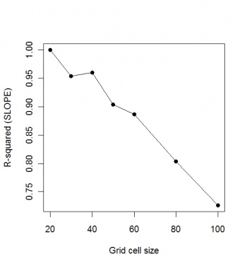
As expected, the difference between the finest resolution SLOPE and coarser resolution SLOPEs will slowly increase (there seems to be no inflection point). From the plot shown below, we can conclude that a resolution of 45 m is still highly similar (R-square >95%) as compared to the 20-meter SLOPE map. A similar type of analysis can be also found in this article.
Selected references
- Atkinson, P.M. and Aplin, P., 2004. Spatial variation in land cover and choice of spatial resolution for remote sensing. Photogrammetric Engineering and Remote Sensing, 25(18): 3687-3702.
- Bishop, T.F.A., McBratney, A.B. and Whelan, B.M., 2001. Measuring the quality of digital soil maps using information criteria. Geoderma, 103(1-2): 95-111.
- Dungan, J.L. et al., 2002. A balanced view of scale in spatial statistical analysis. Ecography, 25: 626-640.
- Florinsky, I.V. and Kuryakova, G.A., 2000. Determination of grid size for digital terrain modelling in landscape investigations – exemplified by soil moisture distribution at a micro-scale. International Journal of Geographical Information Science, 14(8): 815–832.
- Heuvelink, G.B.M. and Pebesma, E.J., 1999. Spatial aggregation and soil process modelling. Geoderma, 89(1-2): 47-65.
- Hutchinson, M.F., 1996. A locally adaptive approach to the interpolation of digital elevation models. In: Proceedings of the Third International Conference/Workshop on Integrating GIS and Environmental Modeling. National Center for Geographic Information and Analysis, Santa Barbara, CA, 6 pp.
- McBratney, A.B., 1998. Some considerations on methods for spatially aggregating and disaggregating soil information. Nutrient Cycling in Agroecosystems, 50: 51-62.
<Rating> Rate this article: 1 Poor and in error 2 Far from ready 3 Needs improvements 4 Minor corrections 5 Very useful!! </Rating>
