Best Combined Spatial Prediction

S

patial prediction (also known as spatial interpolation) is a process of estimating values of some target variable at a new location, using sampled values and auxiliary data (maps) that can be used to explain variation of the target variable. A technique (algorithm) that generates spatial predictions given a set of inputs can be called a spatial prediction method. A common objective of somebody interested to generate quality maps using geostatistics is to compare a variety of spatial prediction methods and then select the one that is: (a) the most accurate (cross-validation), (b) least biased, (c) most robust (sensitivity analysis), (d) most reliable, and (e) fastest possible. There are many spatial predictors described in the literature. The Spatial Interpolation Comparison game, for example, lists over 35 techniques. Sometimes you will discover that there are not as many possibilities. In fact, there are only dozen truly independent spatial predictors (e.g. mechanical, splines-based, kriging-based, regression-based and machine learning-based predictors). Many spatial prediction methods produce fairly similar outputs (even if their names seem to indicate completely different algorithms).

This article demonstrates how to make a quick comparison of the most popular spatial predictors (inverse distances, ordinary kriging, regression-based predictors) implemented in the gstat package (read more on obtaining and installing the software used below). A simple approach is suggested to generate the Best Combined Spatial Prediction using predictions produced variety of methods. This assumes that the predictors are mutually independent and that they address different features of interest.

Sample script to compare spatial predictors.

spatial_predictors_meuse.R : R script to compare various spatial predictors and generate BCSP.

For this purpose we will use the "meuse" dataset provided together with the gstat package:

UNIQ3e6b7784606e07b-geshi-00000000-QINU

Once we have prepared all maps, we can proceed with running predictions. We consider six standard techniques: inverse distances (ID), regression on coordinates (TR), simple linear regression (LM), ordinary kriging (OK), GLM-based regression, and regression-kriging (RK):

UNIQ3e6b7784606e07b-geshi-00000001-QINU

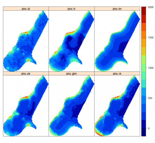
In principle, all techniques can be automated. We can finally plot all predictions next to each other:

UNIQ3e6b7784606e07b-geshi-00000002-QINU

Figure: Comparison of predictors implemented in gstat.

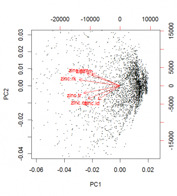
To compare various predictions (maps), we can use the Principal Component Analysis (PCA):

UNIQ3e6b7784606e07b-geshi-00000003-QINU

Figure: Visual comparison of similarities between the predictions produces using six methods. Note that inverse distance interpolation and GLM predictions seem to be the least correlated.

This shows that ID and OK, and LM and GLM are highly correlated (as expected); RK lies in-between (as expected); all predictors are positively correlated (of course).

Different predictors can be also compared by estimating the time needed to generate predictions for all grid nodes:

UNIQ3e6b7784606e07b-geshi-00000004-QINU

In this case the difference is fairly small. In reality (large datasets) some simple local predictor can be few thousands time faster than global predictors.

The Best Combined Spatial Prediction (BSCP) can be produced by combining the predictions of multiple prediction techniques. Assuming that a series of prediction techniques are mutually independent (i.e. they do not use the same model parameters; they treat different parts of spatial variation), the BCSP can be generated as a weighted average from multiple predictions:

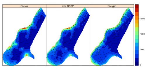
where is the prediction error estimated by the model (prediction variance), and is the number of predictors. For example, in the case study from above (meuse), we can generate a combined prediction using OK and GLM-regression:

UNIQ3e6b7784606e07b-geshi-00000008-QINU

Figure: The BCSP as a combination of OK and GLM-regression (weighted average).

Note that the prediction will in some parts of the study are look more as OK, in others more as GLM, which actually depicts extrapolation areas of both methods (this map is probably very similar to predictions produced using regression-kriging). In general, the map in the middle looks more as the GLM-regression map because this map is about 2-3 times more precise than the OK map (read more about visualization of uncertainty in maps). It is important to emphasize that, in order to combine various predictors, we do need to have an estimate of the prediction uncertainty, otherwise we are not able to assign the weights. In principle, linear combination of statistical techniques using the equation above should be avoided if a theoretical basis exists that incorporates such combination.

In the example above (GLM+OK), we assume that the the predictions/prediction errors are independent, and they are probably not. In addition, a statistical theory exists that supports a combination of regression and kriging (see e.g. Diggle and Ribeiro, 2007), so there is no need to run the predictions separately and derive an unrealistic measure of model error. The BCSP can be only interesting for situations where there are indeed several predictors possible, where no theory exists that reflects their combination, and/or where fitting of individual models is faster and less problematic than fitting of a hybrid model.

The combined prediction error of a BCSP can be estimated by summing up simulated values using the same formula from above. This might be computationally intensive as we need at least 20 simulations to get a reasonable estimate of the additive prediction variance.

---

<Rating> Rate this article: 1 Poor and in error 2 Far from ready 3 Needs improvements 4 Minor corrections 5 Very useful!! </Rating>