Analysis of DEMs in R+ILWIS/SAGA
he science of quantitative analysis of land surface or surfaces in general is refer to as geomorphometry. One of the main objectives of geomorphometry is the (automated) extraction of land-surface parameters and objects, and assessment of their properties. Analysis of DEMs can be today easily automated by combining open source packages R+ILWIS/SAGA (read more on how to obtain and install these packages). This allows us to run series of same operations on DEMs coming from various sources (or on their simulations) and compare the outputs using sound statistical procedures. The complete script used to generate graphs and maps shown below is available here. Note that you can try running the same script using any of the four DEMs attached. These are the DEMs of the same area, but generated using elevation measurements from various data sources (National Elevation Dataset, SRTM DEMs). See also an ArcGIS script to measure drumlin attributes from a DEM. An updated version of this article can be followed in Hengl (2009; ch.9).
|
Contents |
Import of DEMs and extraction of land surface parameters
We start by reading a DEM into R:
> gridmaps <- readGDAL("NED1.asc")  # this scripts uses only one DEM; to compare analysis, change the input!
> names(gridmaps)[1] <- "DEM"
> proj4string(gridmaps) <- CRS("+init=epsg:32618")
> spplot(gridmaps)
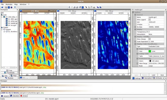
Next, we want to extract Topographic Wetness Index, altitude above channel network and solar insolation. All this can be extracted using the SAGA GIS. We start by converting the DEM (ArcInfo ASCII) to SAGA grid format:
> rsaga.esri.to.sgrd(in.grids="NED1.asc", out.sgrds="NED1.sgrd", in.path=getwd())

# derive catchment area:
> rsaga.geoprocessor(lib="ta_hydrology", module=15, param=list(DEM="NED1.sgrd", C="catharea.sgrd",
+      GN="catchslope.sgrd", CS="modcatharea.sgrd", SB="twi.sgrd", T=10))

# filter the spurious sinks:
> rsaga.geoprocessor(lib="ta_preprocessor", module=2, param=list(DEM="NED1.sgrd", RESULT="NED1_f.sgrd"))

# extract channel network:
> rsaga.geoprocessor(lib="ta_channels", module=0, param=list(ELEVATION="NED1_f.sgrd",
+      CHNLNTWRK="chnlntwrk.sgrd", CHNLROUTE="channel_route.sgrd", SHAPES="channels.shp",
+      INIT_GRID="NED1_f.sgrd", DIV_CELLS=round(sqrt(length(gridmaps@data[[1]]))/100, 0),
+      MINLEN=round(sqrt(length(gridmaps@data[[1]]))/10, 0)))

# derive altitude above channel network:
> rsaga.geoprocessor(lib="ta_channels", module=3, param=list(ELEVATION="NED1_f.sgrd",
+      CHANNELS="chnlntwrk.sgrd", ALTITUDE="achan.sgrd", THRESHOLD=0.1, NOUNDERGROUND=TRUE))

# derive incoming solar radiation:
> rsaga.geoprocessor(lib="ta_lighting", module=2, param=list(ELEVATION="NED1.sgrd",
+      INSOLAT="insolat.sgrd", DURATION="durat.sgrd", LATITUDE=43, HOUR_STEP=4, TIMESPAN=2, DAY_STEP=10))
# ! this can take time; modify latitude accordingly;
We can read the maps back to R:
> rsaga.sgrd.to.esri(in.sgrds=c("twi.sgrd", "achan.sgrd","chnlntwrk.sgrd", "insolat.sgrd"),
+      out.grids=c("twi.asc", "achan.asc", "chnlntwrk.asc", "insolat.asc"), prec=1, out.path=getwd())
> gridmaps$twi <- readGDAL("twi.asc")$band1
> gridmaps$achan <- readGDAL("achan.asc")$band1
> gridmaps$insolat <- readGDAL("insolat.asc")$band1
> gridmaps$chnlntwrk <- readGDAL("chnlntwrk.asc")$band1
Some land-surface parameters are very skewed, so you might want to transform them:
hist(gridmaps$DEM); hist(gridmaps$twi); hist(gridmaps$achan)
gridmaps$logachan <- log1p(gridmaps$achan)
hist(gridmaps$logachan)
Unsupervised extraction of landforms
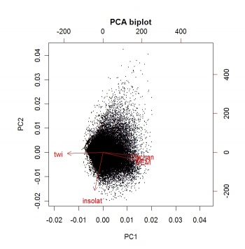
An objective way to extract landform parameters is to use the kmeans method of the stats package in R. Before we actually extract the landforms, it is a wise idea to reduce multicolinearity of the land-surface parameters by running a Principal Component Analysis:
> pc.dem <- prcomp(~DEM+twi+achan+insolat, scale=TRUE, gridmaps@data)
> biplot(pc.dem, arrow.len=0.1, xlabs=rep(".", length(pc.dem$x[,1])), main="PCA biplot")
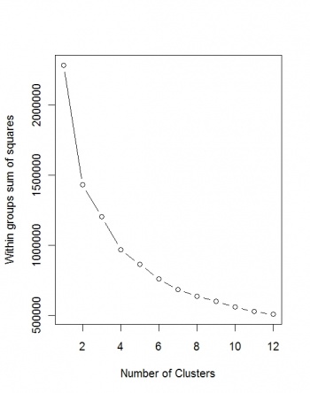
Next, we wish to determine the optimal number of clusters:
> demdata <- as.data.frame(pc.dem$x)
> wss <- (nrow(demdata)-1)*sum(apply(demdata,2,var))
> for (i in 2:12) {wss[i] <- sum(kmeans(demdata, centers=i)$withinss)}
> plot(1:12, wss, type="b", xlab="Number of Clusters", ylab="Within groups sum of squares")
Unfortunately, the Sum of squares does not converge, so we can at least use the maximum number of clusters (12):
> kmeans.dem <- kmeans(demdata, 12)
> gridmaps$kmeans.dem <- kmeans.dem$cluster
> gridmaps$landform <- as.factor(kmeans.dem$cluster)
> summary(gridmaps$landform)
> spplot(gridmaps["landform"], col.regions=rainbow(12))
# writeAsciiGrid(gridmaps["kmeans12.dem"], "landform.asc")
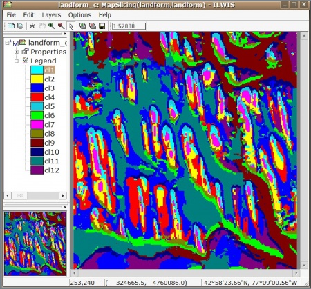
We can write this landform map to ILWIS GIS and display it so we can edit the legends manually:
> writeGDAL(gridmaps["kmeans.dem"], "landform.mpr", "ILWIS")
# create a domain in ILWIS:
> shell(cmd=paste(ILWIS, " crdom landform.dom -type=group -items=0",sep=""), wait=F)
# add elements to the domain:
> for(i in 1:length(levels(gridmaps$landform))){
   shell(cmd=paste(ILWIS, " additemtodomaingroup landform.dom ", i+.01," cl",i,sep=""), wait=F)
}
> shell(cmd=paste(ILWIS, "landform_c.mpr = MapSlicing(landform.mpr, landform.dom)"), wait=F)
> shell(cmd=paste(ILWIS, "open landform_c.mpr -noask"), wait=F)
Supervised classification of land-surface objects
If some training data is available, we can also map a belonging of a certain area to what we have visually classified into a certain class (landform). Imagine that a polygon map is available with borders of some landform of interest (in this case drumlins). We want to use this map to specify the position of the class in feature space, and then derive a probability of drumlin using some relevant land surface parameters. We first need to import this map to R:
# import the map showing location of drumlins (training pixels)
> drumlins <- readShapePoly("drumlins.shp")
# spplot(drumlins)
# overlay drumplins and grid maps and create a new grid:
> gridmaps$drumlins <- as.factor(overlay(gridmaps, drumlins))
Next, we need to estimate the class centres and variation around class centers based on the training areas:
# standard deviation:
> drumlin.var <- sd(subset(gridmaps@data, drumlins=="2")[c("DEM","twi","logachan")], na.rm=T)
> drumlin.var
      DEM       twi  logachan
2.4675426 0.7109454 0.2330179
# mean values:
> drumlin.mean <- mean(subset(gridmaps@data, drumlins=="2")[c("DEM","twi","logachan")], na.rm=T)
> drumlin.mean
       DEM        twi   logachan
177.565516  11.051724   2.318473
# range of values (most reliable):
> drumlin.range <- data.frame(DEM=range(subset(gridmaps@data, drumlins=="2")["DEM"], na.rm=T),
+     twi=range(subset(gridmaps@data, drumlins=="2")["twi"], na.rm=T),
+     logachan=range(subset(gridmaps@data, drumlins=="2")["logachan"], na.rm=T))
> drumlin.range
    DEM  twi logachan
1 174.0  9.8 1.916923
2 182.9 12.5 2.766319
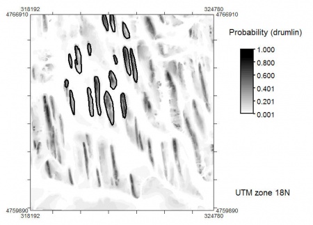
We can now calculate the mean normal density function (probability) that a point belongs to some class in the feature space. In this case, we use the extreme values of DEM, twi and achan, because we assume the class centers are in fact where the elevation is highest; twi is the lowest; and achan is the highest!
> qu <- 2  # adjustment factor!
# average probability:
> gridmaps$drumlin.mu <- (2*pnorm(abs((gridmaps$DEM-drumlin.range[2,"DEM"])/(qu*drumlin.var["DEM"])), lower.tail=F)
+     +2*pnorm(abs((gridmaps$twi-drumlin.range[1,"twi"])/(qu*drumlin.var["twi"])), lower.tail=F)
+     +2*pnorm(abs((gridmaps$logachan-drumlin.range[2,"logachan"])/(qu*drumlin.var["logachan"])), lower.tail=F))/3
# hist(gridmaps$drumlin.mu, breaks=30)
# spplot(gridmaps["drumlin.mu"], col.regions=grey(rev(seq(0,1,0.01))))
# writeGDAL(gridmaps["drumlin.mu"], "mu_drumlin.mpr", "ILWIS")
which gives the following map:
Export of maps to Google Earth
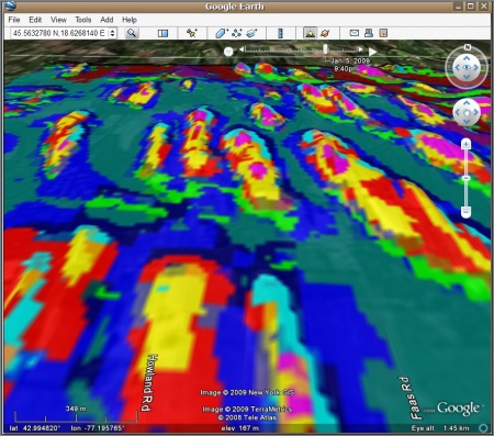
In the last step, we can export the created maps to Google Earth for visual assessment. First, we need to create the grid in the geographic system:
> gridmaps.ll <- spTransform(gridmaps["landform"], CRS("+proj=longlat +datum=WGS84"))
> corrf <- (1+cos((gridmaps.ll@bbox[2,2]+gridmaps.ll@bbox[2,1])/2*pi/180))/2
> geogrd.cell <- corrf*(gridmaps.ll@bbox[1,2]-gridmaps.ll@bbox[1,1])/gridmaps@[email protected][1]
> geoarc <- spsample(gridmaps.ll, type="regular", cellsize=c(geogrd.cell,geogrd.cell))
> gridded(geoarc) <- TRUE
> gridparameters(geoarc)
   cellcentre.offset     cellsize cells.dim
x1         -77.23152 0.0002932871       283
x2          42.97029 0.0002932871       220
Next, we can resample the map to the new geographic grid (e.g. in ILWIS GIS):
> shell(cmd=paste(ILWIS, " crgrf geoarc.grf ",geoarc@[email protected][[2]],"
+     ",geoarc@[email protected][[1]]," -crdsys=LatlonWGS84 -lowleft=(",geoarc@[email protected][[1]],",
+     ",geoarc@[email protected][[2]],") -pixsize=",geoarc@grid@cellsize[[1]],sep=""), wait=F)
> shell(cmd=paste(ILWIS, "landform_ll.mpr = MapResample(landform_c.mpr, geoarc, NearestNeighbour)"), wait=F)
> shell(cmd=paste(ILWIS, "export tiff(landform_ll.mpr, landform_ll.tif)"), wait=F)
Finally, we generate a KML (ground overlay) by using the kmlOverlay method of the maptools package:
> overlay.kml <- GE_SpatialGrid(geoarc)
> kmlOverlay(overlay.kml, "landform.kml", "landform_ll.tif", name="Landform classes")
For more details on how to export raster maps to Google Earth, read also this article.
Important references
- Brenning, A., 2008. Statistical Geocomputing combining R and SAGA: The Example of Landslide susceptibility Analysis with generalized additive Models. In: J. Böhner, T. Blaschke & L. Montanarella (eds.), SAGA - Seconds Out (Hamburger Beiträge zur Physischen Geographie und Landschaftsökologie, 19), 23-32.
- Burrough, P.A., van Gaans, P.F.M.,MacMillan, R.A., 2000. High-resolution landform classification using fuzzy k-means. Fuzzy Sets and Systems 113, 37–52.
- Fisher, P.F., Wood, J., Cheng, T., 2005. Fuzziness and ambiguity in multi-scale analysis of landscape morphometry. In: Petry, F.E., Robinson, V.B., Cobb, M.A. (Eds.), Fuzzy Modeling with Spatial Information for Geographic Problems. Springer-Verlag, Berlin, pp. 209–232.
- Hengl, T. 2009. A Practical Guide to Geostatistical Mapping, 2nd Edt. University of Amsterdam, www.lulu.com, 291 p. ISBN 978-90-9024981-0
- Hengl, T., Reuter, H.I. (eds) 2008. Geomorphometry: Concepts, Software, Applications. Developments in Soil Science, vol. 33, Elsevier, 772 pp. ISBN: 978-0-12-374345-9
- Iwahashi, J., Pike, R.J., 2007. Automated classifications of topography from DEMs by an unsupervised nested-means algorithm and a three-part geometric signature. Geomorphology 86 (3–4), 409–440.
<rating> Rate this article: 1 Poor and in error 2 Far from ready 3 Needs improvements 4 Minor corrections 5 Very useful!! </rating>
