Regression-kriging guide
urpose of this small guide is to help you run regression-kriging (RK) with your own data, using a variety of software packages. I will use a simple case study - interpolation of sampled measurements (100 locations) of soil thickness using a single auxiliary predictor (slope map) - assuming you will be able to extend this case to your own data with multiple predictors and much larger number of sampling and prediction points. The dataset and methodology used are explained in detail in Hengl et al. (2004). Note that regression-kriging is known by different names in different packages. All packages listed bellow in fact implement the so-called Kriging with External Drift algorithm, where both the regression and the residual part of the prediction model are solved simultaneously. Read more about theoretical grounds of regression-kriging in this article.
|
Contents |
gstat (stand-alone)
Gstat (Pebesma, 2004) is probably the best and fastest choice to run RK with your data. You only need to download the exe file from the www.gstat.org website and put it in some directory e.g. c:\gstat\. It is advasible to set an environmental variable under Windows > Control panel > System > Advanced > Environmental variables > Add new variable 'gstat' with value "c:\gstat\" or wherever your exe file is.
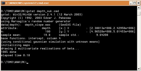
INSTRUCTIONS: 1. Copy the point data file (depth_slope.eas), the auxiliary map (slope.asc) and the gstat command file (depth_uk.cmd) to the working directory; 2. Start DOS prompt by typing: "cmd" in the start> run > menu on your desktop; 3. Move to the active directory using cd.. e.g. cd c:/gstat; 4. Run the gstat programme together with a specific gstat command file from the DOS prompt e.g.:
c:\gstat\gstat depth_uk.cmd
this will do universal kriging using the 'slope.asc' as the predictor (base) map. Note that the commands in gstat are very simple and straight forward. The results will be writen directly to the ArcInfo Ascii format, so that you can visualize the results in most GIS packages. You can modify the input parameters, variogram model etc by editing the gstat command file. For example, the following script can be used to run conditional simulations with 'slope.asc' as the predictor (base) map:
# Interpolation of depth with the help of slope.asc map
# computationally demanding to speed up, limit to neighbourhood of 50 closest points (usually good enough)
# the results of interpolation are writen directly in the common GIS format

points(depth): 'depth_slope.eas',x=1,y=2,v=3,X=4,max=50;
variogram(depth): 34 Nug(0) + 72 Exp(8500);
mask: 'slope.asc';
method: gs;
predictions(depth): 'depth_suk.asc';

# set the number of simulations:
set nsim=2;

# to run block-kriging instead of point kriging just un-mark this line:
# blocksize: dx=100, dy=100;
and this script can be used to automatically fit a variogram:
# automated variogram fitting for residuals
# replace variable number and name in the document

data(depth): 'depth_slope.eas', x=1,y=2,v=5;

# set initial variogram

variogram(depth): 0 Nug(0) + 4 Exp(2000);

# fit the variogram automatically

method: semivariogram;
set fit=7;

# write down the fitted variogram model and gnuplot

set output= 'var_depth.cmd';
set plotfile= 'var_depth.plt';
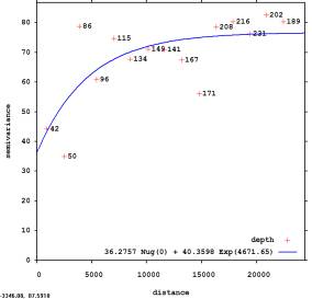
You can then view the resulting plot using wgnuplot. Note that, for automated modeling of variogram, you will need to define an initial variogram then is then fitted against the true values. As initial variogram, you can set nugget parameter = 0, sill parameter = sampled variance and range = 10% of spatial extent of the data. Make sure you also consult the gstat user's manual. A problem with gstat is that you need to have regression residuals before you run interpolation, so you will anyway need to do some regression analysis before preparing the gstat command file. Note also that the simulations with base maps in gstat can be quite time-consuming. In principle, the creator of gstat has stopped maintaining the stand-alone version of gstat (although it might be relatively faster to run the stand-alone version than to run universal kriging in R+gstat; there are also no memory limit problems if you use the stand-alone version). Thus you should really consider using gstat within R.
R+gstat
R is an open-source environment for statistical computing and visualization. It is based on the S language and is the product of an active movement among statisticians for a powerful, programmable, portable, and open computing environment, applicable to the most complex and sophisticated problems. R for MS Windows (you will need version 2.0 or higher) you can download and install in few minutes. After the installation, you should also install and load packages gstat, sp and rgdal. Read more about how to install necessary packages.
INSTRUCTIONS: In R, raster and vector maps can be imported in two ways: a) point maps (DEPTH.txt) you can import as tables first, then converted to SpatialPointsDataFrame:
> library(sp)
> library(lattice)
> trellis.par.set(sp.theme()) # for blue-pink-yellow color ramp
> depth <- read.delim("DEPTH.txt")
> str(depth)
'data.frame':   100 obs. of  3 variables:
 $ X    : int  2412518 2412764 2416694 2412207 2413458 2422209 ...
 $ Y    : int  4970823 4969523 4969656 4970518 4980254 4966624 ...
 $ DEPTH: int  25 18 20 22 12 25 ...
> coordinates(depth)=~X+Y
> str(depth)
Formal class 'SpatialPointsDataFrame' [package "sp"] with 5 slots
  ..@ data       :'data.frame': 100 obs. of  1 variable:
  .. ..$ DEPTH: int [1:100] 25 18 20 22 12 25 18 22 8 18 ...
  ..@ coords.nrs : int [1:2] 1 2
  ..@ coords     : num [1:100, 1:2] 2412518 2412764 2416694 2412207 2413458 ...
  .. ..- attr(*, "dimnames")=List of 2
  .. .. ..$ : NULL
  .. .. ..$ : chr [1:2] "X" "Y"
  ..@ bbox       : num [1:2, 1:2] 2380132 4965281 2429583 5014533
  .. ..- attr(*, "dimnames")=List of 2
  .. .. ..$ : chr [1:2] "X" "Y"
  .. .. ..$ : chr [1:2] "min" "max"
  ..@ proj4string:Formal class 'CRS' [package "sp"] with 1 slots
  .. .. ..@ projargs: chr NA
b) the raster map (slope.asc) you can import from ArcInfo ASCII format by using the sp package:
> slope <- read.asciigrid("slope.asc", as.image=FALSE, plot.image=TRUE)
> str(slope)
Formal class 'SpatialGridDataFrame' [package "sp"] with 6 slots
  ..@ data       :'data.frame': 40000 obs. of  1 variable:
  .. ..$ slope.asc: num [1:40000] 45.5 34.3 19.3 12.5 13.4 17.2 21.2 ...
  ..@ grid       :Formal class 'GridTopology' [package "sp"] with 3 slots
  .. .. ..@ cellcentre.offset: num [1:2] 2380000 4965000
  .. .. ..@ cellsize         : num [1:2] 250 250
  .. .. ..@ cells.dim        : int [1:2] 200 200
  ..@ grid.index : int(0)
  ..@ coords     : num [1:2, 1:2] 2380000 2429750 4965000 5014750
  .. ..- attr(*, "dimnames")=List of 2
  .. .. ..$ : NULL
  .. .. ..$ : chr [1:2] "coords.x1" "coords.x2"
  ..@ bbox       : num [1:2, 1:2] 2379875 4964875 2429875 5014875
  .. ..- attr(*, "dimnames")=List of 2
  .. .. ..$ : chr [1:2] "coords.x1" "coords.x2"
  .. .. ..$ : chr [1:2] "min" "max"
  ..@ proj4string:Formal class 'CRS' [package "sp"] with 1 slots
  .. .. ..@ projargs: chr NA
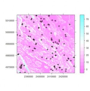
> spplot(slope, scales=list(draw=T), sp.layout=list("sp.points", depth, pch="+"))
This plot shows that we are dealing with a point map consisting of 100 points and a slope map consisting of 40,000 grids.
Note that R is not a GIS package so that (geo)visualisation options are very limited (although the new sp package show significant number of new GIS capabilities). To interpolate sampled variable DEPTH using KED/UK and SLOPE as predictors, you need to run the following steps:
1. Fit and plot the regression model:
> slope.ov = overlay(slope, depth)   # create grid-points overlay
> depth$slope.asc =slope.ov$slope.asc   # copy the slope values

> lm.depth <- lm(DEPTH~slope.asc, depth)
> summary(lm.depth)

Call:
lm(formula = DEPTH ~ slope.asc, data = as.data.frame(depth))

Residuals:
      Min        1Q    Median        3Q       Max
-19.09701  -6.19463   0.04989   5.15362  24.71945

Coefficients:
            Estimate Std. Error t value Pr(>|t|)
(Intercept) 25.28709    1.31779  19.189  < 2e-16 ***
slope.asc   -0.41037    0.07537  -5.445 3.84e-07 ***
---
Signif. codes:  0 ‘***’ 0.001 ‘**’ 0.01 ‘*’ 0.05 ‘.’ 0.1 ‘ ’ 1

Residual standard error: 8.491 on 98 degrees of freedom
Multiple R-squared: 0.2323,     Adjusted R-squared: 0.2244
F-statistic: 29.65 on 1 and 98 DF,  p-value: 3.84e-07

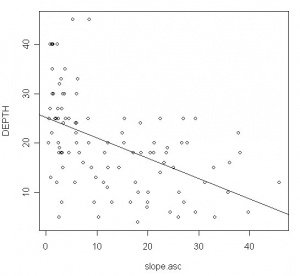
> plot(DEPTH~slope.asc, as.data.frame(depth))
> abline(lm(DEPTH~slope.asc, as.data.frame(depth)))
2. Estimate the residuals and their autocorrelation structure (variogram):
> library(gstat)
> null.vgm <- vgm(var(depth$DEPTH), "Sph", sqrt(areaSpatialGrid(slope))/4, nugget=0) # initial parameters
> vgm_depth_r <- fit.variogram(variogram(DEPTH~slope.asc, depth), model=null.vgm)
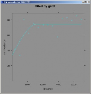
> plot(variogram(DEPTH~slope.asc,depth), vgm_depth_r, main="fitted by gstat")
3. Run KED/UK:
> depth_uk <- krige(DEPTH~slope.asc, locations=depth, newdata=slope, model=vgm_depth_r)
[using universal kriging]

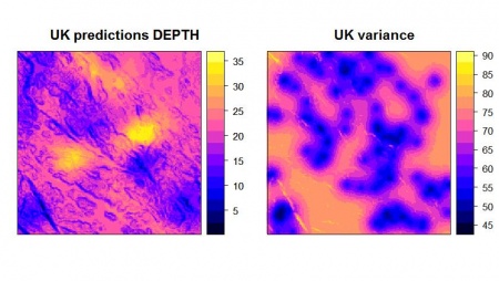
> print(spplot(depth_uk, "var1.pred", main="UK predictions DEPTH"), split=c(1,1,2,1), more=T)
> print(spplot(depth_uk, "var1.var", main="UK variance"), split=c(2,1,2,1), more=F)
This will plot final predictions with appropriate legend and title. After you run KED/UK in gstat, you can export the results of interpolation and import them back to a GIS package using the rgdal package:
> write.asciigrid(depth_uk[1], "DEPTH_UK.asc")
this makes an array of grid nodes in ArcInfo Ascii format.
To run geostatistical simulations instead of predictions, simply add an extra argument:
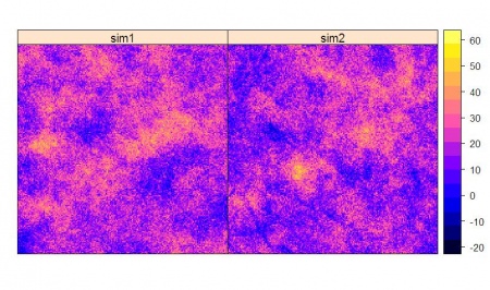
> depth_suk <- krige(DEPTH~slope.asc, locations=depth, newdata=slope, model=vgm_depth_r, nsim=2, debug.level=-1)
drawing 2 GLS realisations of beta...
[using conditional Gaussian simulation]
> spplot(depth_suk)
You can also run regression and kriging of residuals separately and then sum the outputs:
> depth_rk <- krige(DEPTH~slope.asc, locations=depth, newdata=slope)  # regression part only!
> depth_rok <- krige(residuals(lm.depth)~1, locations=depth, newdata=slope, model=vgm_depth_r)  # OK of residuals
> depth_rk$var1.rk <- depth_rk$var1.pred + depth_rok$var1.pred
> spplot(depth_rk, "var1.rk", main="RK predictions DEPTH")
The advantage of separating regression and kriging part is in possibility to speed up the computations (read more about this topic in this article). Also note that gstat accepts only linear models in form Z~Q. To use non-linear models, please also consider using the geoRglm package.
Idrisi+gstat
Idrisi is one of the GIS packages with largest numbers of raster and vector operations. The price per a single licence is about $600, but you can always order a 7-day evaluation version to test it. In Idrisi, gstat code has been also adjusted and integrated within.
INSTRUCTIONS: First you need to import the two maps using:
- Import > Software-specific-formats > ESRI formats > ARCRASTER (Arcinfo ASCII format to raster) for the slope.asc map; Import > Software-specific-formats > ESRI formats > SHAPEIDR (Shape file to Idrisi ) for the depth.shp map. NOTE: You can use the croatia.ref georeference system instead of the "plane" reference system (download to C:\IDRISI Kilimanjaro\Georef\ directory; see also: Coordinate systems used in ex Yugoslavia). You should first display the two maps using the display launcher.
- You can then model variogram in Idrisi using the Spatial dependence modeller. After you derived semivariances, save and load them in the variogram model fitting environment, where you can (interactively) estimate the variogram model parameters.
- After you finished fitting the variogram, you can save the variogram parameters and load them later to do kriging or simulations.
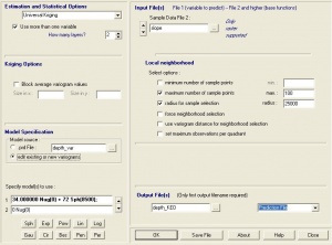
After you fitted the variogram model, you can interpolate the DEPTH map with SLOPE map as auxiliary predictor by: GIS analysis > Surface analysis > Interpolation > Kriging and simulations. You will then get an user-friendly kriging dialog window where you can define: variogram model, variable to predict, auxiliary maps etc. In IDRISI, only raster input files are allowed for input maps. The first input file contains the sample data, the second, third etc input file is a fully sampled surface that has attribute values for all prediction locations. This means that, before runing KED/UK in Idrisi, you need to convert the point map (depth.vct) to a raster image using the RASTERVECTOR operation. Note that a local neighborhood must be specified for each input file. Unfortunately, Idrisi help warns that the Spatial Dependence Modeler can not calculate generalized least squares residuals, although this was originally implemented in gstat. Also note that Idrisi uses term "residuals" with somewhat different meaning - the system will not derive residuals for you but you have to do it by yourself. The final predictions are quite similar to the one produced in R+gstat. Use of gstat within a GIS package is possible also within GRASS and PCRaster (for more info check gstat homepage).
Isatis
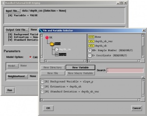
Isatis is the most expensive package (over 10K €) used in this comparison, but is definitively one of the most professional geostatistical packages for environmental sciences. Isatis was originally built for Unix, but there are MS Windows and Linux versions also.
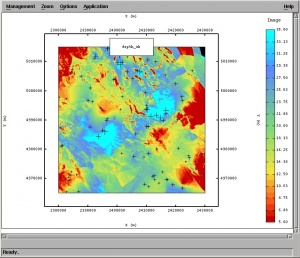
INSTRUCTIONS: In Isatis, you also need to import the point and raster maps first: vector maps can be imported as shape files and raster maps as ArcView ASCII grids (importing/exporting options are limited to standard GIS formats). Note that you first need to define the project name and working directory using the data file manager. After you imported the two maps, you can visualize them using the display launcher.
RK in Isatis is achieved using Interpolation > Estimation > External Drift (Co)-kriging. Here a user needs to select the target variable (point map), predictors and the variogram model. Note that KED in Isatis is limited to only one (three when scripts are used) auxiliary raster map (in Isatis called background variable)! Isatis justifies limitation of number of auxiliary predictors by computational efficiency. In any case, a user can first run factor analysis on multiple predictors and then select the most significant component, or simply use the regression estimates as the auxiliary map. Isatis gives option to fit the variogram model automatically, with or without nugget effect. User can also edit the Model Parameter File where the characteristics of the model you wish to apply for kriging is stored. The user manual does not give insight into the algorithm used (except for the mathematical proofs), so I could not tell how exactly are the KED weights estimated and is there any regression modeling involved prior to the interpolation of data. You finally get predictions that are more similar to ordinary kriging.
SAGA GIS
SAGA (System for Automated Geoscientific Analyses) is a full-fledged GIS with support for raster and vector data, which includes a large set of geoscientific algorithms, being especially powerful for the analysis of DEMs. With the release of version 2.0 in 2005, SAGA works under both Windows and Linux operating systems. In addition, SAGA is an open-source package, which makes it especially attractive to users that would like extend or improve the existing modules. In the most recent version of SAGA (2.0.3), the authors have implemented ordinary and universal kriging with automated fitting of variograms (this means that you only need to select the input rasters and the point map). Unfortunately, SAGA does not support all standard (positive-definite) variogram models such as exponential or Gaussian, which might frustrate advanced users. SAGA also does not support geostatistical simulations nor co-kriging, indicator kriging etc.
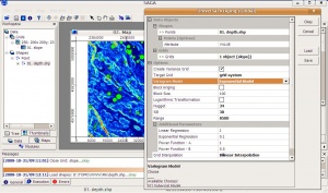
To install SAGA, just download the zip file and extract it under your /Program files/ folder. Regression-kriging is available in SAGA in the module "Geostatistics" under "Universal kriging". The users can select global and local (search radius) version of the Universal kriging. In this case, I do not recommend the use of local Universal kriging because it over-simplifies the technique and can lead to serious artifacts (neither local variograms nor local regression models are estimated). In SAGA, you can also run multiple regression prediction using grids, then derive the residuals and fit the variogram of residuals.
INSTRUCTIONS:
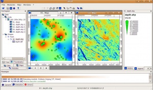
- Copy the shape file (depth.zip), the auxiliary map (slope.asc) in a working directory. You can display the two maps over each other.
- Select Modules > Geostatistics > Kriging > Universal kriging (global) and you will get this menu. Note that you can select as many predictors as you wish, as long as they are all in the same grid system;
- The final results can be visualized in both 2D and 3D spaces.
Note that SAGA can also be run from R using the RSAGA package. This allows you to speed up interpolation of large data sets / maps.
