Who's onlineThere are currently 0 users and 6 guests online.
User loginBook navigationNavigationLive Traffic MapNew Publications
|
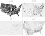
Fig. 6.4. Examples of environmental predictors used to interpolate HMCs.
library(maptools)
library(rgdal)
# Download and extract grids:
download.file("http://spatial-analyst.net/book/system/files/usgrids5km.zip", destfile=paste(getwd(), "usgrids5km.zip", sep="/"))
grid.list <- c("dairp.asc", "dmino.asc", "dquksig.asc", "dTRI.asc", "gcarb.asc", "geomap.asc", "globedem.asc",
"minotype.asc", "nlights03.asc", "sdroads.asc", "twi.asc", "vsky.asc", "winde.asc", "glwd31.asc")
for(j in grid.list){
fname <- zip.file.extract(file=j, zipname="usgrids5km.zip")
file.copy(fname, paste("./", j, sep=""), overwrite=TRUE)
}
# plot the predictors:
library(adehabitat)
image(as.kasc(list(geomap=import.asc("geomap.asc"), nlights03=import.asc("nlights03.asc"),
dTRI=import.asc("dTRI.asc"), gcarb=import.asc("gcarb.asc"))))
|
Latest image Testimonials"From a period in which geographic information systems, and later geocomputation and geographical information science, have been agenda setters, there seems to be interest in trying things out, in expressing ideas in code, and in encouraging others to apply the coded functions in teaching and applied research settings." PollRandom image and gstat (right): regression-kriging.") |
 | Contact: Tomislav Hengl ([email protected]) |
Recent comments
5 years 23 weeks ago
5 years 40 weeks ago
5 years 49 weeks ago
6 years 9 weeks ago