ASTER import

Radiometric and geometric corrections (technical information)

Introduction

ASTER (Advanced Spaceborne Thermal Emission and Reflection Radiometer) images are files written in the Earth Observation System Hierarchical Data Format (EOS-HDF) format, which is a type of the HDF4 file format. An ASTER image is acquired by three different telescopes and contains 15 bands:

• 4 Visible and Near-Infra Red (VNIR) bands with a ground resolution of 15 meters;
• 6 ShortWave Infra Red (SWIR) bands with a ground resolution of 30 meters, and;
• 5 Thermal Infra Red (TIR) bands with a ground resolution of 90 meters.

The individual ASTER bands have the following properties:

Notes:

• ILWIS ASTER Import supports the HDF4 format but does not support the HDF5 format.
• Data acquired in ASTER VNIR bands 3N (Nadir looking) and 3B (Backward looking) can be used to create a Digital Elevation Model (DEM).

Tip:

Detailed information on the ASTER sensor can currently be found at http://asterweb.jpl.nasa.gov/instrument.asp.

ILWIS ASTER import supports two types of ASTER images:

• ASTER level 1A files
• ASTER level 1B files

The level 1A raw data are reconstructed, unprocessed instrument digital counts. This product contains image data with geometric correction coefficients and radiometric calibration coefficients appended but not applied. This includes correcting for SWIR parallax as well as registration within and between telescopes. The spacecraft ancillary and instrument engineering data are also included. The radiometric calibration coefficients consisting of offset and sensitivity information is generated from a database for all detectors. The geometric correction is the coordinate transformation for band-to-band registration.

The level 1B product contains radiometrically calibrated and geometrically coregistered data for all channels. This product is created by applying the radiometric and geometric coefficients to the level 1A data. After that the radiances are scaled back to DN values making use of a single calibration coefficient "Linc" for each band (see formula 3). The bands have been coregistered both between and within the telescopes, and the data have been resampled to apply the geometric corrections. As for level 1A products these level 1B radiances are generated at 15 meter, 30 meter and 90 meter resolutions corresponding to the VNIR, SWIR and TIR channels. Calibrated, at-sensor radiances are given in Wm^-2sr^-1�m^-1. Level 1B data is path oriented and destriping and bad pixel replacement have been applied.

Tip:

Detailed information about the ASTER products can currently be found at http://asterweb.jpl.nasa.gov/data_products.asp.

Radiometric Corrections

The Digital Numbers in a ASTER level 1A file are values describing the voltage output of a sensor mapped within a suitable range (0-255 for the VNIR and SWIR channels and 0-4094 for the TIR channels). These raw DN values can be converted to an actual physical value, called radiance (in Wm^-2sr^-1�m^-1), using the corrections of the radiometric correction table that is embedded in the HDF file. Radiometrically correcting the ASTER level 1A image will remove, as far as possible the striping (slight systematic differences in DN values between adjacent columns in the map) caused by different characteristics of the sensors. When applying radiometric corrections two cases have to be handled:

• correction for VNIR and SWIR bands, and;
• correction for TIR bands.

The VNIR and SWIR bands use a pushbroom sensor technology so that each line will be captured in full by an array of 4100 sensors. The radiometric correction has to be applied for each of the 4100 sensors. The formula used in ILWIS to convert the raw DN values of each individual VNIR and SWIR band to radiance values (L) is:

where:

The TIR bands use a whiskbroom technology so another correction is needed. Blocks of an image are scanned in a 10 x 700 matrix that moves across the scene (70 blocks). Each of the 10 lines in a block has a separate set of parameters for radiometric correction. For each individual TIR band the formula to convert DN values to radiance values (L) is:

where:

Notes:

• Even after the radiometric correction process some striping may remain as the radiometric correction table may diverge from the actual correction needed. A filter may be required to further remove striping.
• All calculations for radiometric correction will use a precision of 0.001.
• The user may want to convert radiance values back to sensor calibrated DN values. These sensor calibrated DN values are not the actual digital unprocessed numbers of the file but radiometric corrected radiance values scaled back into an appropriate range using the formula:

  DNcalibrated = L/C

  formula 3

  where:

  DNcalibrated	= sensor calibrated DN value
  L	= calculated radiance value
  C	= unit conversion coefficient; a linear scale factor for each band read from the meta data in the HDF file

An ASTER level 1B file already contains radiometrically calibrated DN values. The formula used in ILWIS to convert these radiometrically calibrated DN values to radiance values (L) is:

where:

Output

Geometric corrections

Geometrical knowledge of the imported ASTER bands is defined by the Georeference (relation between pixel RowCol positions and plane XY coordinates) and the Coordinate System parameters (either geographic or geodetic LatLons or projected map coordinates).

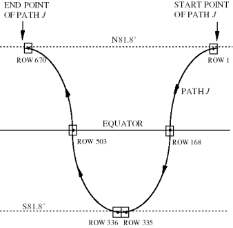
ASTER level 1A data contains sets of tiepoints with given geocentric LatLons on the WGS84 spheroid. The Aster User�s Guide Version 3.1 Part 1, March/June 2001 gives formulas to convert them to geodetic LatLons, at least for the center of each scene. The following calculations are carried out when importing an ASTER image. The results are found under the Additional Info of the created UTM coordinate system.

The geocentric latitude PSI for scene number K is calculated as (Aster User's Guide Part 1, March 2001):

where:

The geocentric latitude PSI found in the HDF file can be converted into the geodetic (WGS84) latitude PHI using the following formula (Aster User's Guide Part 1, March 2001):

where:

The longitude in the center of the scene can be found from the scene number K and the path number J using the following formulas:

The longitude L_K=168,J of the descending node at the Equator for the path J can be expressed as follows:

The longitude L_K,J of row K and path J can be expressed as follows:

For the descending path:

For the ascending path:

where:

The LatLon tiepoints of ASTER level 1A are converted to Universal Transverse Mercator (UTM) coordinates of the appropriate zone, similar to what is done for ASTER level 1B data. However for the level 1A data the full set of tiepoints available in the HDF file and a 3^rd order transformation are used.

Note:

The number of tiepoints is variable depending on the telescope.

ASTER level 1B data contains images already resampled to the geometry of the appropriate UTM projection with the WGS84 Datum. The images are however not north-oriented but path-oriented. ILWIS creates for this purpose a georeference with the 4 corners as tiepoints

The tiepoints coordinates (in UTM) can be obtained from the lattice of 13 X 11, 107x104 and 12x11 LatLons given for respectively VNIR, SWIR and TIR, simply by applying the relevant projection transformation. The applicable UTM zone can be found in the metadata of the HDF file.

Output

Notes:

The georeferences for ASTER level 1B are the same per sensor group (VNIR, SWIR and TIR) except VNIR band 3B which has a separate one.

Tips:

• With the Epipolar Stereo Pair operation you can create a stereo pair from the two ASTER bands VNIR 3N and VNIR 3B.
• The Coordinate System Properties sheet gives additional information that can be relevant in case of mosaicking ASTER images. The Additional Info tab gives information about:
  Zone:
  Central Meridian:
  Scale Factor at Central Meridian:
  Geographic area:
  Latitude limits: rMinLat, rMaxLat
  Longitude limits: rMinLon, rMaxLon
  Scene (Row-) Number: iSceneNr 
  Orbit Path Number: iPathNr 
  Geocentric Latitude at Row SceneNr
  Geodetic Latitude at Row SceneNr
  Longitude at Row SceneNr

See also:

Import ASTER

Import Map