Horton statistics

Functionality

The Horton Statistics operation calculates for all streams with a certain (Strahler) stream order number i, located in merged catchment C with ID x:

Cx_N: the number of streams,
Cx_L: the average stream length (km),
Cx_A: the average area of catchments (km²),

Cx_N_LSq: expected values for Cx_N by means of a least squares fit through Cx_N,
Cx_L_LSq: expected values for Cx_L by means of a least squares fit through Cx_L,
Cx_A_LSq: expected values for Cx_A by means of a least squares fit through Cx_A.

The output is stored in a table which can be used to construct so-called Horton plots in a graph window.

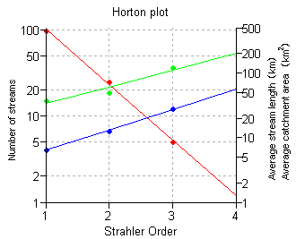
Horton plots enable you to inspect the regularity of your extracted stream network based on the (Strahler) stream order numbers, and may serve as a quality control indicator for the entire stream network extraction process. It is expected that:

the number of streams show a relative decrease for subsequent Strahler order numbers,
the length of streams and the catchment areas show a relative increase for subsequent Strahler order numbers,

For more information on the actual creation of Horton plots, see the section Construction of Horton plots in a graph window below.

Input map requirements:

the output raster map and its linked attribute table of a previous Catchment extraction operation,
the output raster map and its linked attribute table of a previous Catchment merge operation,
the output raster map and its linked attribute table of a previous Drainage network ordering operation.

Domain of output table:

A new ID domain will be created for the output table. The domain obtains the same name as the output table itself. The domain contains the Strahler order numbers as IDs.

Example of output table:

When you used a merged catchment map containing a single catchment, and when the maximum Strahler Order value in your Drainage network ordering output table equals 4, the output table of the Horton Statistics operation may look like follows:

Columns starting with C represent the merged catchment(s); records represent the Strahler stream order numbers.

Note: the Cx_N_LSq, , Cx_L_LSq, Cx_A_LSq columns are currently incorrectly named: Cx_RB, Cx_RL, Cx_RA.

Columns in the output table:

If your merged catchments map contains more than a single catchment, the last three columns exist for every catchment; x represents a catchment number.

domain	The IDs of the table's domain, every record (ID) represents a certain Strahler order number.
Order	The Strahler order numbers as values. This column usually contains the same values as the IDs of the table.
Cx_N	The number of streams with a certain Strahler stream order number.
Cx_L	The average length (km) of the streams with this Strahler order number.
Cx_A	The average area (km²) of the catchments belonging to the streams with this Strahler order number.

Cx_N_LSq	The expected number of streams with a certain Strahler stream order number.
Cx_L_LSq	The expected average length (km) of the streams with this Strahler order number.
Cx_A_LSq	The expected average area (km²) of the catchments belonging to the streams with this Strahler order number.

Tip: To calculate R_B, R_L, or R_A values for subsequent order numbers, or for the regression lines, please refer to Horton Statistics : algorithm.

Implementation of Least Squares Fit within a Horton output table:

When the total number of stream orders, i.e. the number of records in the Horton table, is � 2, a least squares fit will not be calculated.
When the total number of stream orders equals 4, the highest order is ignored during the least squares fit (i.e. values in the last record will not be taken into account).
When the total number of stream orders is ³ 5, the lowest and highest orders are ignored during the least squares fit (i.e. values in the first and the last record in the table will not be taken into account.)

Construction of Horton plots in a graph window

The general idea is to construct a graph:

with on the X-axis the Strahler stream order numbers,
on a left logarithmic Y-axis:
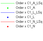
- the number of streams per order number (C1_N), as points,
- the expected values for the number of streams per order number by Least Squares Fit (C1_N_LSq), as a line,
on a right logarithmic Y-axis:

the average stream length per order number (C1_L), as points,
the expected values for the average stream length per order number by Least Squares Fit (C1_L_LSq), as a line,
the average catchment area per order number (C1_A), as points,
the expected values for the average catchment area per order number by Least Squares Fit (C1_A_LSq), as a line.

An example of Horton plots is shown below.

Suppose you only had a single catchment in your merged catchments map.

Open the output table to create the graphs. In the table window, choose File, Create, Graph ...

Add the points for the number of streams C1_N:

In the Create Graph dialog box:

accept the name of the current table,
for the X-axis, accept the Order column,
for the Y-axis, choose the C1_N column.

Adapt the Y-axis:

From the Graph Management pane, double-click Y-axis left:

in the Y-axis (left) dialog box: choose a Logarithmic axis type.
adapt the minimum and maximum values for the axis if required.

Add the expected values C1_N_LSq:

From the Edit menu in the Graph window, choose Add Graph from Columns, or click the Add Graph button in the toolbar of the graph window.
In the Add Graph from Columns dialog box:

accept the name of the current table,
for the X-axis, accept the Order column,
for the Y-axis, choose the C1_N_LSq column.

Initially, this will be displayed as points in yellow...

Adapt the drawing of the expected values to a line graph and adapt the color to the same color as the points with empirical values:

From the Graph Management pane, double-click the graph layer Order x C1_N_LSq:
In the Graph Options - Graph from Columns dialog box:

choose Line,
choose the same color as you used for the empirical point values C1_N from step 1.

Repeat steps 1 to 4 above for the empirical stream length values Order x C1_L, and expected stream length values Order x C1_L_LSq.
Make sure that these values are bound to a right-hand, logarithmic Y-axis.

Repeat steps 1 to 4 above for the empirical catchment area values Order x C1_A, and expected catchment area values Order x C1_A_LSq.
Make sure that these values are bound to a right-hand, logarithmic Y-axis.

The Horton plots will then look like follows:

Reference:

Ven te Chow, D.R. Maidment, L.W. Mays (1988) Applied hydrology. In: McGraw-Hill Series in Water Resources and Environmental Engineering. McGraw-Hill, New York. pp. 166-170. ISBN 0-07-010810-2.